Climbing trees 1: what are decision trees?

This is the first in a series of posts about decision trees in the context of machine learning. The goal here is to provide a foundational understanding of decision trees and to implement them.

Decision trees are not amazing algorithms by themselves. They have limitations that can result in suboptimal and even weird predictions. And yet, they have become extremely popular. Some would even say they are the de facto go-to algorithm for many machine learning domains. This is due to bagging and boosting, techniques that turned subpar decision trees into state-of-the-art algorithms. We’ll explore them in the future.

First, we’ll build an intuition for what are decision trees and define them mathematically. Then, we’ll explore how decision trees are built. This will allow us to grasp their main characteristics, advantages and disadvantages. I will try to introduce complexity gradually, but I will assume you have some knowledge on mathematical notation, statistics and basic machine learning concepts.

If things become too complicated, try to read the provided references. I’ve drawn upon various sources instrumental to my understanding of decision trees, including books, documentation, articles, blog posts and lectures. Even if you understand everything, check the references: there is great content there.

What is a decision tree?

Imagine you’re trying to decide whether to take an umbrella when leaving home. You might ask questions like: “Are there clouds?”. If yes, you might then ask “What’s the humidity level?”. Each question helps you narrow down the decision. This is how a decision tree works.

Let’s simulate this weather example:

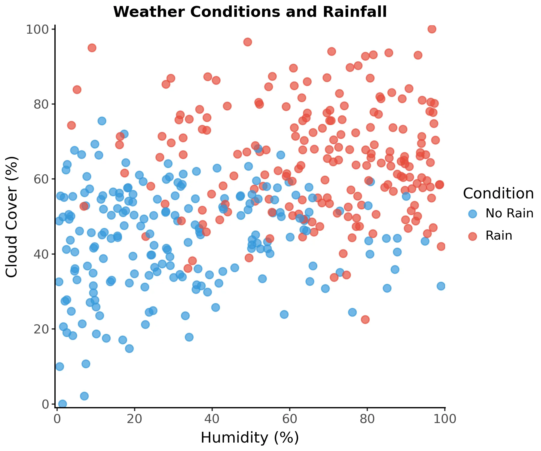
Scatter plot of humidity and cloud coverage showing that it's more likely to rain when its cloudy and humid

A decision tree can be thought of as making consecutive decisions by asking a series of questions about our data. Each internal tree node uses a certain feature (in our example, cloud cover or humidity) to divide its region into two using a split value. Each new region can be further divided into two. A node that divides its region into two is called an internal node.

Leaf (or terminal) nodes don’t ask any more questions, but rather provide a prediction for its region. In our example, it might say “Rain” or “No rain”. More precisely, it assigns a probability for each outcome.

Let’s take a look at a decision tree fitted to our weather example:

Graph of decision tree splits

This decision tree was kept intentionally small. From top to bottom, this graph represents all decision boundaries of our simple tree. Each internal node produces two branches, that is, two paths that can be followed. These branches recursively partitions the feature space such that the samples with the same labels or similar target values are grouped together. For instance, we predict that it’ll rain if humidity is above 59% and cloud cover is above 45% (rightmost path in the graph) because most points (instances) in this region are of the “Rain” class.

The class shown is only relevant for leaf nodes, that is, those at the bottom row. The value property shows how many samples there are for each class in each region. A pure node has only instances of one class in its region. Since all nodes contain at least one instance of both classes (that is, “Rain” and “No Rain”), all nodes are impure. The objective during training is to reduce impurity as much as possible. If all nodes are pure, then the tree has zero error on the training data set. This is how decision trees learn.

This visualization of the tree is very easy to interpret. We can follow each path and clearly see why a prediction was made, that is, the model is easily explainable (the opposite of a black-box model). This is one of the reasons why decision trees are popular. Simple decision trees can even be applied in some practical settings (e.g. medicine) without machine assistance.

We can also visualize the decision boundaries of the tree by overlaying them onto the scatter plot of our data:

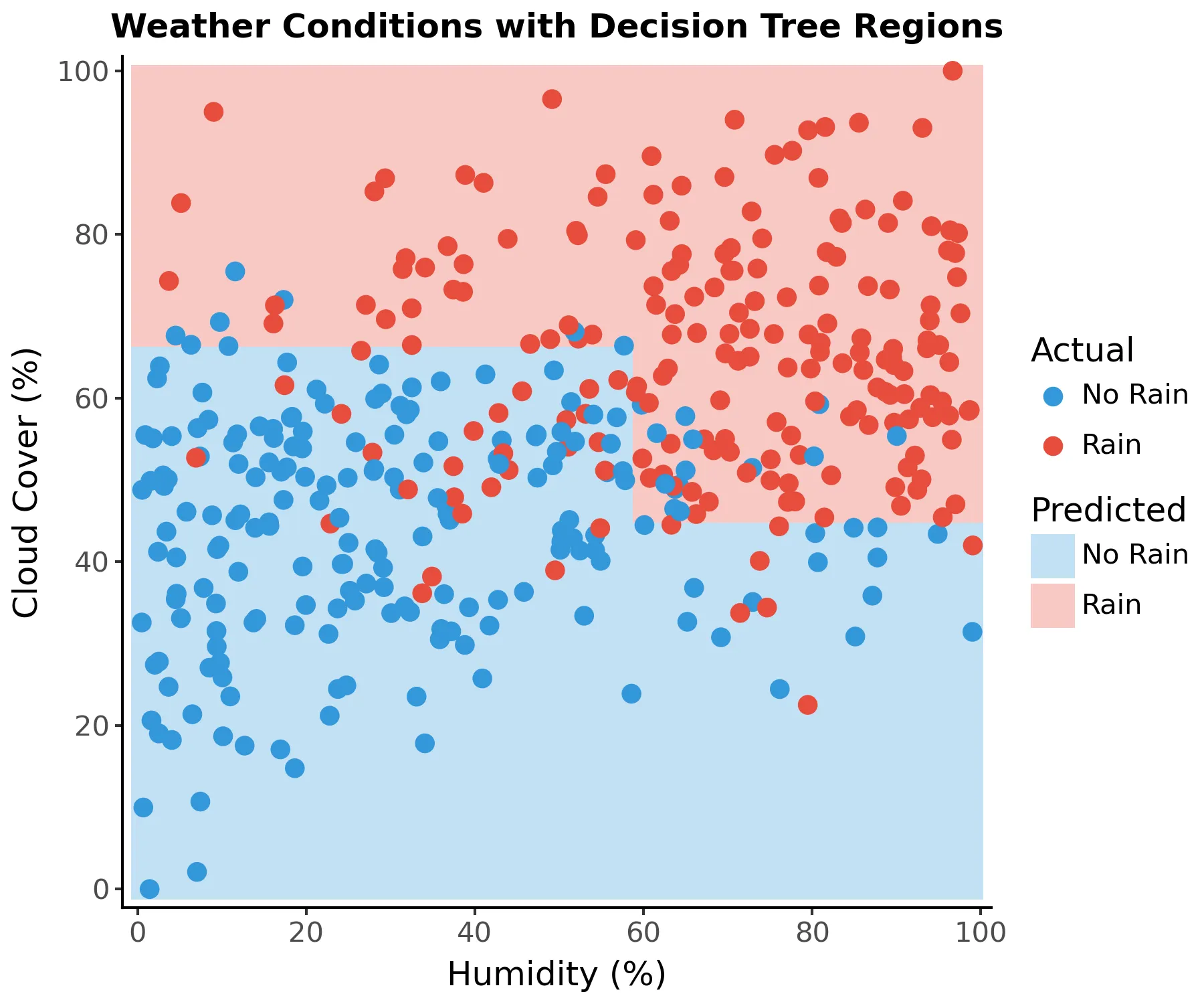
Scatter plot of humidity and cloud coverage showing prediction regions from a decision tree

We can see the straight boundaries between regions. More formally, a decision tree is a hierarchical structure that recursively divide our features into cuboid regions. Since we have 2 features (2 dimensions) in our example, the cuboid regions are squares.

Types of trees

Broadly, there are two types of decision trees: classification and regression trees. While they share the same fundamental structure and splitting methodology, they differ in their output and how they make predictions.

Classification trees are designed to predict categorical outcomes — they assign input data to predefined classes or categories. At each leaf node, the tree predicts the most common class among the training samples that reached that node. Our weather example involves a classification tree and the leaves predict whether it will rain or not. The prediction is made by counting the proportion of training samples of each class at the leaf node and selecting the majority class. Think of it as the tree asking a series of yes/no questions about the input features until it can make an educated guess about which category the input belongs to.

Regression trees, on the other hand, predict continuous numerical values rather than categories. Instead of predicting a class at each leaf node, regression trees typically output the average value of all training samples that reached that node. For instance, a regression tree might predict a house’s price based on features like square footage, number of bedrooms, and location. Each split in the tree tries to group together similar numerical values. When a new example comes in, the tree can guide it to a leaf node containing training examples with similar target values and use their average as the prediction.

Decision tree algorithms

Decision trees have been widely explored and there is a wide range of different decision tree algorithms. The most influential ones are ID3 (Iterative Dichotomiser 3), C4.5 and CART (Classification and Regression Trees).

ID3 is one of the earliest decision tree algorithms and support only classification with categorical features. Nodes can be split into more than two depending on the number of categorical levels of each feature.

C4.5 extends the ID3 algorithm to support numerical features and missing values. CART is similar to C4.5 but also adds support for regression.

The CART approach only performs binary splits, resulting in taller trees when compared to ID3 and C4.5. Although the principles discussed here apply to most decision tree algorithms, I am focused on CART — which is also the algorithm we’ll implement.

Mathematical definition

Mathematically, a decision tree can be described as:

f(x) = \sum_{m=1}^{M} c_m \mathbb{I}(x \in R_m)

Where $x$ are the input features, $R_m$ is the $m$ ‘th region and $c_m$ is the value of this region. $\mathbb{I}(x \in R_m)$ is 1 if $x$ is contained in the $m$ ‘th region, 0 otherwise. The values ( $c$ ) are typically a constant (regression) or a vector of probabilities (classification). The combination of regions and values defines the decision tree.

The regions cannot assume arbitrary boundaries, though. They are always parallel to some axis and can only divide a previous region. This can be a limitation, but it greatly reduces the computational complexity of constructing a decision tree. In our weather example, it’s trivial to find the following decision boundary using other methods (I have used logistic regression):

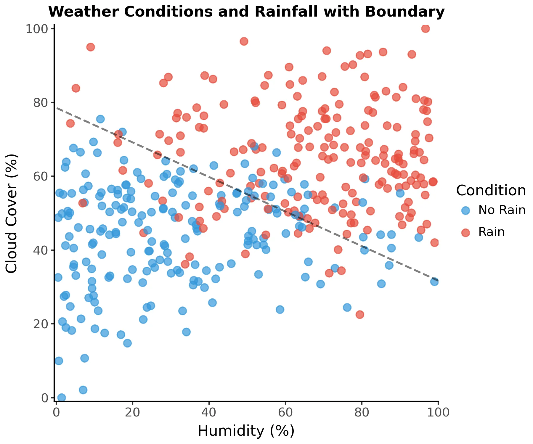
Weather scatter plot with diagonal decision boundary

However, axis-parallel splits (single feature) are much easier to compute than oblique splits (multiple features). Finding the best split of a single feature involves sorting the data and evaluating splits. Since the latter is negligible compared to sorting, this operation has a time complexity of $O(n \log n)$ , where $n$ is the number of data points. To find the best oblique split combining two features, however, we must first consider all possible $O(n^2)$ lines formed by pairs of points. For each line, you need to evaluate which side each point falls on: $O(n)$ . This amounts to a total time complexity of $O(n^3)$ . More generally, an oblique split has a time complexity of $O(n^{d+1})$ , in which $d$ is the number of features. Therefore, we compromise on using only axis-parallel splits, which define cuboid regions.

Each region $R_m$ is defined by a path from the root to the $m$ ‘th leaf of the tree. For instance, consider the path that defines the region $R = \{(Humidity,\ Cloud)\ |\ Humidity > 59\ \text{and}\ Cloud > 45\}$ .

Path between the root node and a leaf node

This region can be visualized on the scatter plot:

Defined region in scatter plot

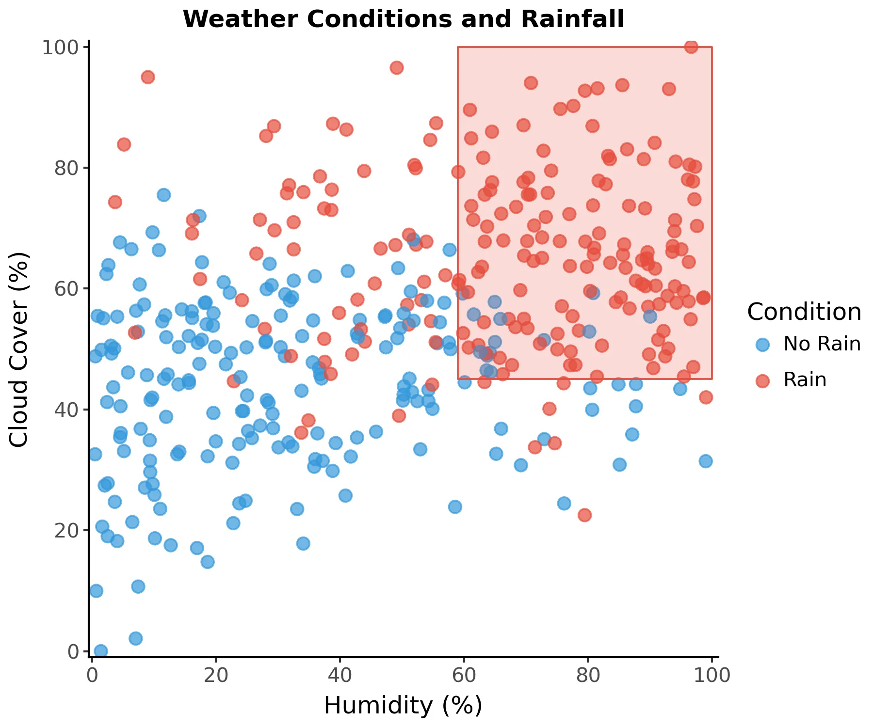
Unlike linear models, decision trees do not model the entire data distribution. Rather, each region has independent predicted values. More formally, adding all independent regions defines a piecewise function that can approximate any pattern in the data, but it may struggle to represent smooth or continuous functions properly.

Bias-variance tradeoff

As all other machine learning algorithms, trees are also haunted by the bias-variance tradeoff. If this concept is new to you, I highly recommend reading about it first (check the references), but come back later.

Bias-variance tradeoff refresher

In summary, bias refers to the error that a model makes due to oversimplification of relationships between features (underfitting). Variance measures how sensitive model predictions are to small fluctuations in the training set. High variance means that the model is capturing noise rather than true relationships (overfitting). Reducing bias tends to increase variance and vice-versa. Finding an optimal bias-variance balance is crucial to achieve good prediction accuracy.

Decision tree variance

Due to the non-linear and non-smooth nature of trees, they easily capture noise. Thus, deeper trees present more variance. If you fully grow a tree, it will partition the feature space until the error is zero¹. The model will have effectively memorized the training set — including noise — which results in overfitting.

If we rebuild our example tree until the error is 0 we get the following regions:

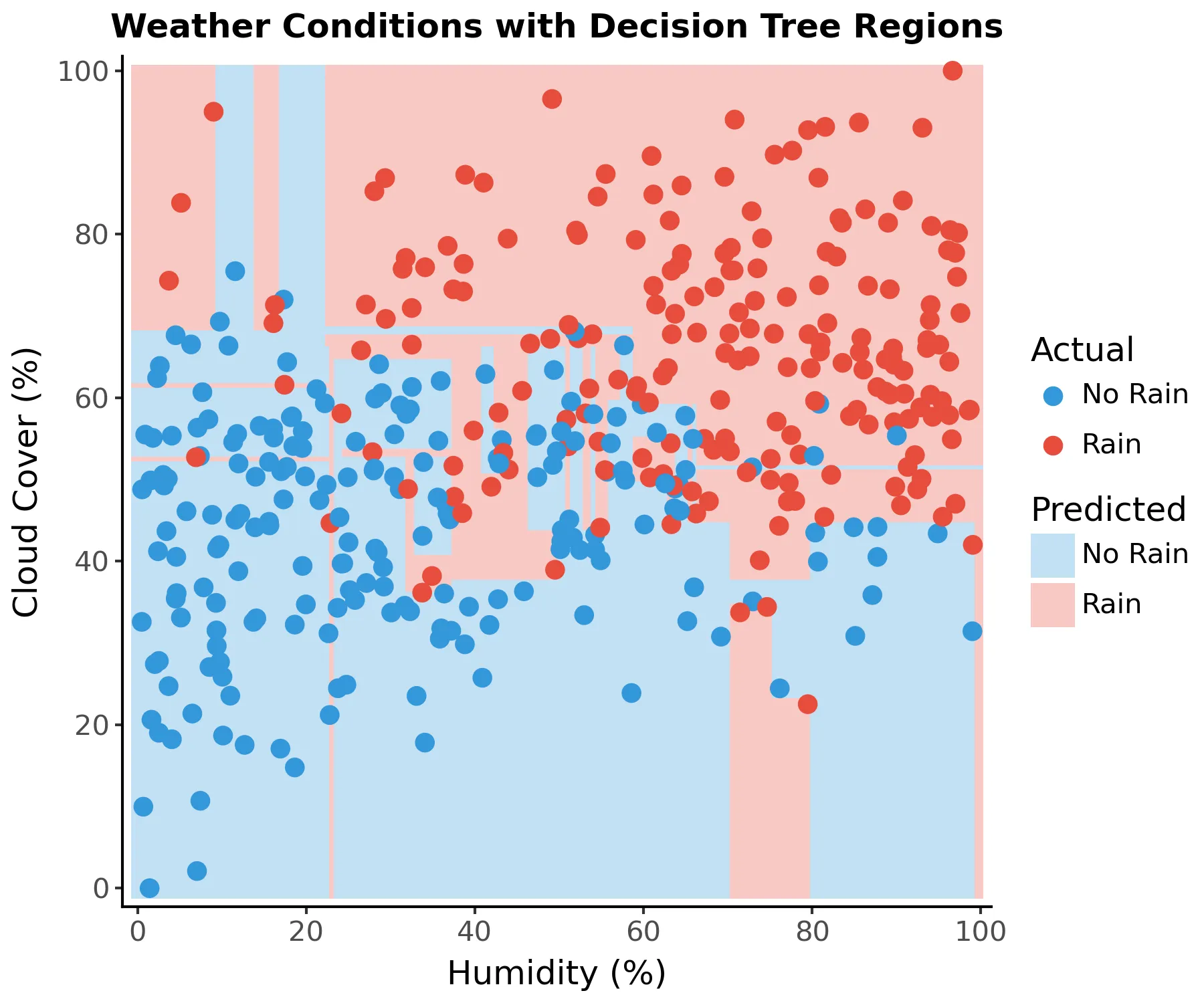
Scatter plot of humidity and cloud coverage showing prediction regions from a deep decision tree

It has perfect accuracy, but it has very unusual boundaries due to noise (high variance). This model doesn’t generalize well, that is, it would score poorly with new data. There are different ways to limit tree variance, namely:

Limiting depth
Requiring a minimum number of points per node
Requiring a minimum decrease in loss to split the node (usually not a good idea)

The number of samples required to fill a tree doubles for each additional level (depth) of the tree. These limits ensure leaf nodes are not overly sparse. Another possibility is to fully grow the tree and later prune it to balance complexity and accuracy.

Let’s build decision trees with increasing depths on a toy dataset:

Depth: 1

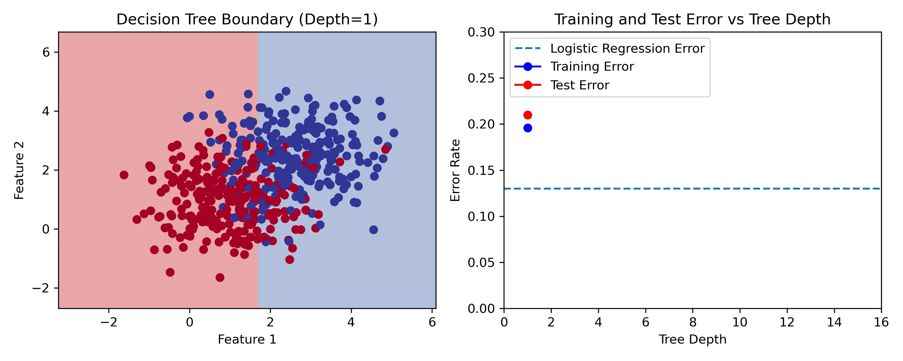
On the left we can see the training set² with two features and two classes. We’re building classification trees, whose decision boundary is overlaid onto the left plot. The plot on the right shows training and test error, as well as the test error of a logistic regression model as a baseline. The test set was sampled from the same distribution, but is different from the training set. Use the slider to compare depths. We can see that the best test error happens with a depth of 3. Increasing the depth further results in overfitting.

Decision tree bias

Even with a depth of three in the example above the error is larger than the logistic regression baseline. This is an example where linear models outperform decision trees due to the additive structure of the data. The logistic regression equation in this case is:

logit(p) = \beta_{0} + \beta_{1} x_{1} + \beta_{2} x_{2} + \varepsilon

Where $p$ is the probability of the outcome being of class 1. Ignoring constants and the noise ( $\varepsilon$ ), the probability is determined by a linear combination of both features. The relationship between features is not hierarchical, therefore decision trees require multiple, sometimes redundant, splits to approximate this concept, leading to deep or overly complex trees.

There are other concepts that fall under the same category, such as:

XOR (Exclusive OR): the output is of one class if exactly one (but not both) of two inputs is true.
Parity problem: the output is different if the number of true values in a set of inputs is even or odd.
Multiplexer problem: a multiplexer selects one of several input values based on a separate “selector” input.

These may seem overly specific, but they’re used as benchmarks to test the capabilities machine learning algorithms. Additive structure, XOR and parity involve global dependencies that require multiple inputs to be considered together. Decision trees split data based on one feature at a time, therefore are inefficient at capturing these relationships. Multiplexer problems require conditional rules which are not hierarchical, making the tree very large to account for all combinations of selector-input pairs.

In more complex real-world datasets, it’s quite likely that multiple non-hierarchical concepts are present, leading to suboptimal bias. If they have subpar variance and bias, decision trees may look like a poor choice of algorithm. Indeed, they rarely shine on their own, but rather as ensembles (with bagging or boosting), which we’ll cover in the future.

The staircase effect

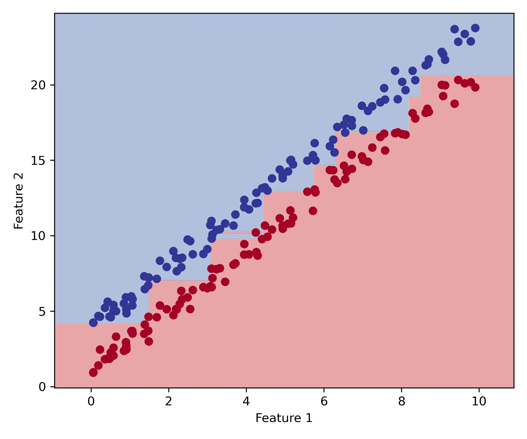
When decision trees attempt to model additive structure, they face a structural constraint that is common enough for me to name it the “staircase” effect³. This limitation manifests differently in classification and regression tasks, but stems from axis-aligned splits.

In classification problems, the staircase effect becomes apparent when the optimal decision boundary between classes involves a linear combination of features (an oblique boundary). Consider a simple case where the optimal boundary is a diagonal line in a two-dimensional feature space. Because decision trees can only make splits parallel to the feature axes, they must approximate this diagonal boundary through a series of rectangular regions, creating a stair-like pattern.

Demonstration of the staircase effect in classification

In regression settings, the staircase effect is even more prominent because regression trees must approximate continuous functions using discrete, constant-valued regions. When the underlying relationship is smooth — whether linear, polynomial, or any other continuous function — the tree’s prediction surface has a stair-like structure with abrupt changes between adjacent regions. Increasing tree depth approximates the prediction surface to the training set, yet the surface does not necessarily become smooth as it captures feature noise.

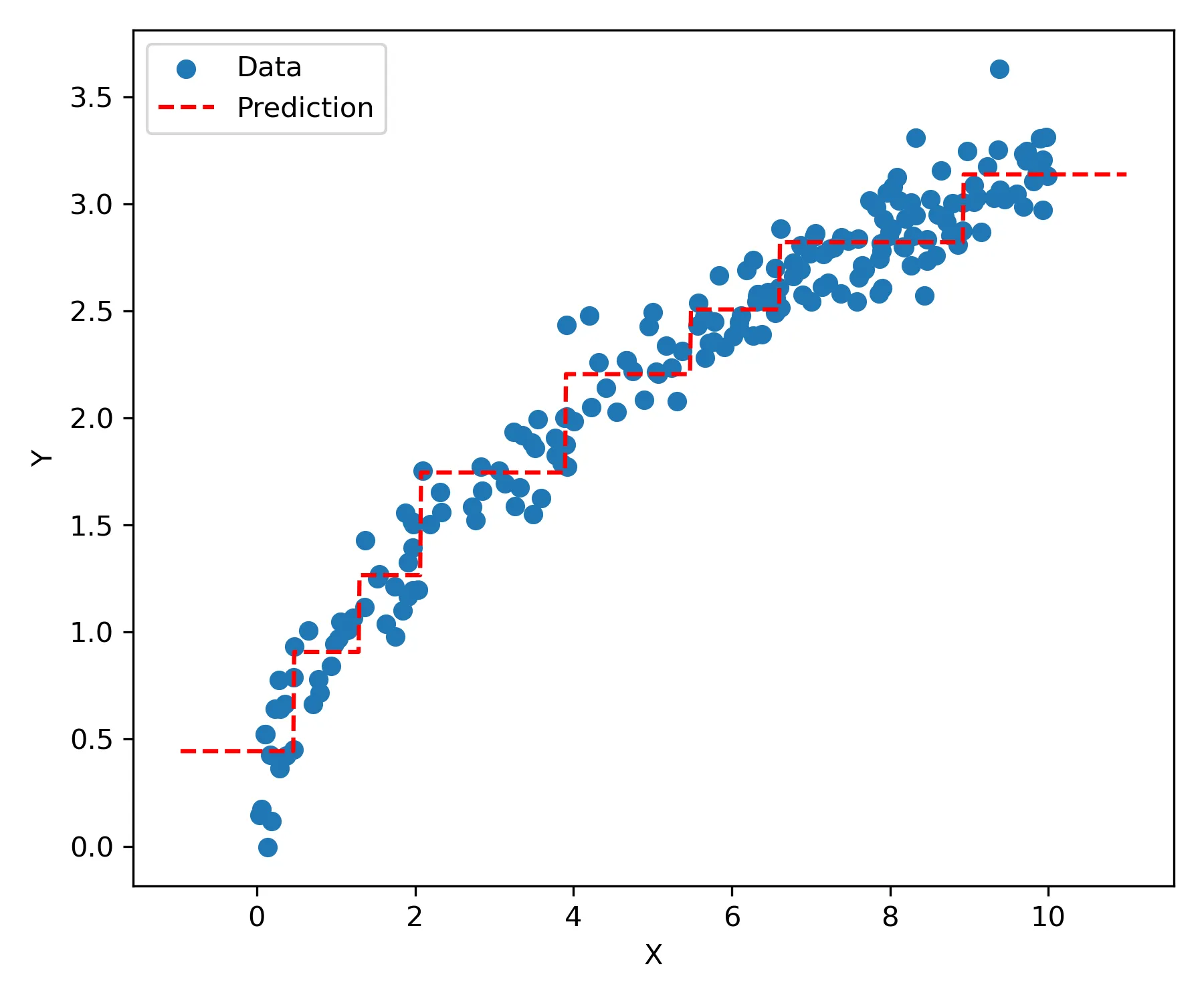
Demonstration of the staircase effect in regression

Regression example with the staircase effect. There is only one feature ( $x$ ) and the vertical axis is the outcome.

Objective functions

We need to define objective functions to optimize for during training. Classification trees use either Gini impurity or entropy as objective functions. Regression trees usually use the squared loss.

In all examples, consider the data $\mathcal{D} = \{(x_1, y_1), ..., (x_n, y_n)\}, y_i \in \{1, ..., c\}$ where $c$ is the number of classes.

Misclassification rate

MR(\mathcal{D}) = \frac{\sum_{i=1}^n \mathbb{I}(\hat{y}_i \neq y_i)}{n}

This is a very intuitive objective for classification. It measures the proportion of misclassified examples. The prediction $\hat{y}$ is the majority vote of the node. Our goal is to decrease leaf node impurity, which is aligned with the misclassification rate function.

Gini impurity

The Gini impurity⁴ over a set of class probabilities $p$ is defined as:

G(\mathcal{D}) = \sum_{k=1}^{c} p_{k}(1 - p_{k}) = 1 - \sum_{k=1}^c p_{k}^2

It measures how often a randomly chosen element of a set would be incorrectly labeled if it were labeled randomly and independently according to the distribution of labels in the set. When the node is pure, one class has a probability of 1 and the rest 0, so the Gini impurity is also 0. The worst Gini impurity arises when the probabilities are uniform among classes, that is, a node with maximum Gini impurity is no better than a coin toss at classifying examples. It can be shown that the upper bound of Gini impurity is 1 as the number of classes grow.

To evaluate the quality of a split ( $\mathcal{S}$ ), we calculate the Gini impurity of each child node and take the weighted average.

G(\mathcal{D}|\mathcal{S}) = \frac{|\mathcal{D}_L|}{|\mathcal{D}|} G(\mathcal{D}_L) + \frac{|\mathcal{D}_R|}{|\mathcal{D}|} G(\mathcal{D}_R)

Where $\frac{|\mathcal{D}_L|}{|\mathcal{D}|}$ is the fraction of inputs in the left child node and $\frac{|\mathcal{D}_R|}{|\mathcal{D}|}$ , in the right.

Entropy

H(\mathcal{D}) = - \sum_{k=1}^{c} p_{k}\ log_{2} p_{k}

The entropy criterion is a concept from information theory (Shannon entropy). It measures the average level of uncertainty of a set of probabilities. In other words, it’s the expected amount of information required to describe the potential outcomes. When probabilities are uniformly distributed entropy is maximum, just like Gini impurity. To understand the connection between information and probabilities, consider you have a set with two classes that are equally likely (let’s say red and blue). If you draw a sample, you have the least possible amount of certainty about which color you’ve drawn. On the other hand, if red has a 95% probability, you can be pretty confident about which color you’ll draw — this has much lower uncertainty. When probabilities are uniform you need extra information to accurately convey the result of a series of draws.

The range of the entropy criterion is from 0 to $log_{2}(c)$ . We also take the weighted average of child nodes to evaluate the quality of a split:

H(\mathcal{D}|\mathcal{S}) = \frac{|\mathcal{D}_L|}{|\mathcal{D}|} H(\mathcal{D}_L) + \frac{|\mathcal{D}_R|}{|\mathcal{D}|} H(\mathcal{D}_R)

It’s also common to see the objective function expressed in terms of information gain, which is the decrease in entropy yielded by a node split.

IG(\mathcal{D}) = H(\mathcal{D}) - H(\mathcal{D}|\mathcal{S})

It represents the amount of information gained about our target variable given our split. In these terms, the objective is to maximize information gain.

Comparing classification objectives

Although misclassification rate is intuitive and commonly used as a model metric, it’s not used as an optimization objective. We can come up with splits ( $\mathcal{S}$ ) that have the same misclassification rate, but one has a pure node while the other doesn’t. For instance:

\mathcal{S} = \{A: 10, B: 0\},\ \{A: 10, B: 5\}

\mathcal{S}' = \{A: 10, B: 2\},\ \{A: 10, B: 3\}

Both splits misclassify 5 samples of class B (same misclassification rate), however the first has a pure node. From an optimization perspective, we should favor pure nodes as they reduce the number of subsequent splits. You can check that indeed both the entropy and the Gini impurity of the second split are higher.

Checking that the affirmation holds

Misclassification rate:

MR(\mathcal{D}|\mathcal{S}) = \frac{10}{25} 0 + \frac{15}{25} \frac{5}{15} = 0.2

MR(\mathcal{D}|\mathcal{S}') = \frac{12}{25} \frac{2}{12} + \frac{13}{25} \frac{3}{13} = 0.2

MR(\mathcal{D}|\mathcal{S}) = MR(\mathcal{D}|\mathcal{S}')

Gini impurity:

G(\mathcal{D}|\mathcal{S}) = \frac{10}{25} 0 + \frac{15}{25} 0.444 = 0.266

G(\mathcal{D}|\mathcal{S}') = \frac{12}{25} 0.277 + \frac{13}{25} 0.355 = 0.318

G(\mathcal{D}|\mathcal{S}) < G(\mathcal{D}|\mathcal{S}')

For the same reason, a tree may get “stuck” when there is no split that minimizes the misclassification rate. Gini impurity and entropy consider probabilities, while misclassification rate considers only the majority vote and therefore is not sensitive enough.

More formally, both Gini impurity and entropy are strictly concave functions. If you take two points on the curve of a strictly concave function and draw a line between them, the line will be always below the curve.

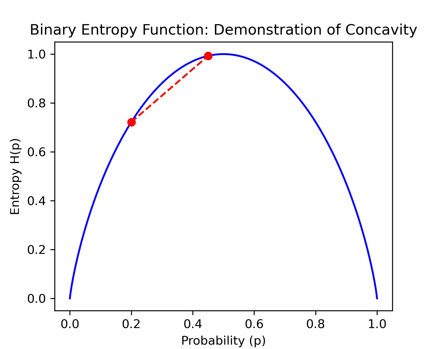
Plot of the entropy function with a line segment below the curve

Plot of entropy $H(p)$ over probabilities $p$ with two classes. The probability of the second class is $(1 - p)$ .

We know from the data processing inequality that the average entropy cannot increase after a split. Either a split reduces entropy in both child nodes — which results in lower average entropy compared to the parent node — or one child node has higher entropy than the parent node and the other lower. Both child nodes cannot have higher entropy than the parent node because this would mean that the split created new information (uncertainty), violating the data processing inequality. Thus, we only need to show that the average entropy decreases when one child node has higher entropy and the other lower compared to the parent node. The strict concavity of the entropy function is enough to ensure this.

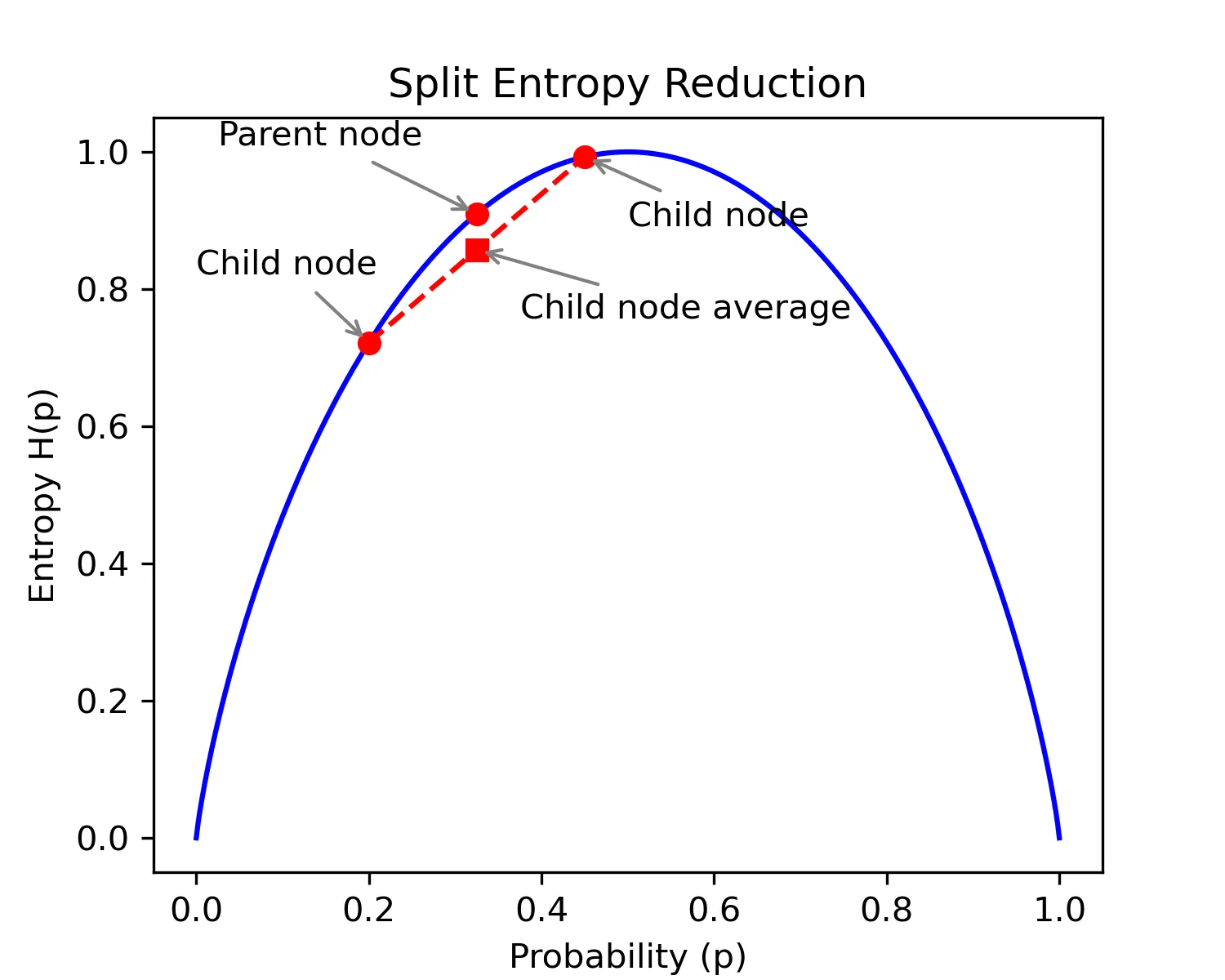
Plot of entropy over probabilities showing labeled node points

The average child node entropy lies somewhere along the line between the points of both child nodes in the curve. The average probability must be the same of the parent node, so the average child node entropy always lies directly below the parent node entropy. Hence, there is ~~almost~~⁵ always a split which results in a lower child node average entropy.

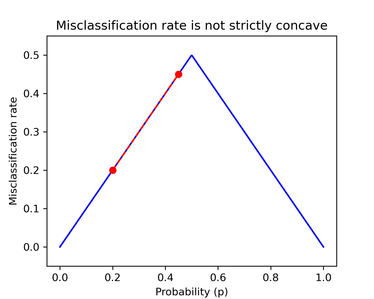
Misclassification rate is not strictly concave. The average misclassification rate of child nodes is equal to that of the parent node when both child nodes lie on the same side of the function, halting the optimization process.

Plot showing line segment over misclassification rate function

Squared loss

L(\mathcal{D}) = \frac{1}{N} \sum_{i=1}^N (y_{i} - \bar{y})^2

The squared loss function is the primary optimization criterion for regression trees. In this equation, $\bar{y}$ represents the mean value of the target variable $y$ within a specific node. This value becomes the prediction ( $c$ ) for all observations that fall into that node, following the mathematical definition of decision trees.

While this formula resembles the traditional mean squared error (MSE) used in many statistical applications, there is an important distinction. In standard regression models, MSE typically measures the difference between predictions ( $\hat{y}$ ) and actual values, where $\hat{y}$ can be directly optimized through model parameters. However, in the context of decision trees, this squared loss function actually quantifies the within-node variance of the target variable.

This variance interpretation leads to an intuitive understanding of the tree-building process: the algorithm seeks splits that maximize the reduction in variance between the parent node and its children. This approach, often termed variance reduction, effectively partitions the data into increasingly homogeneous subgroups with respect to the target variable. The optimal split is one that creates child nodes with minimal average variance, thereby improving the tree’s predictive accuracy.

Building a decision tree

A sufficiently large tree will have one training sample per node, effectively memorizing the training set. Such tree achieves 0 training error, but it is a pathological optimization case. Our goal is to build the smallest possible tree that achieves 0 training error. If limits such as maximum depth are enforced, we should find the tree that minimizes the objective while respecting such limits.

Unfortunately, the computational complexity grows combinatorially and finding the optimal tree is NP-complete. It would be nice to build trees before the heat death of the universe, so we proceed with a greedy algorithm. We make a series of locally optimal choices, hoping that it leads to a solution somewhat close to the global optimum.

Let’s build a classification tree using the Gini impurity criterion. Starting with all of the data and the first variable, we test all possible split points ( $N - 1$ splits) and choose the one with the lowest criterion. Then, we repeat this procedure with all other features. The split with the lowest criterion over all features is chosen. Finally, we repeat the procedure for the left and right child nodes recursively until the criterion is 0 in all nodes or until a tree size limit is reached.

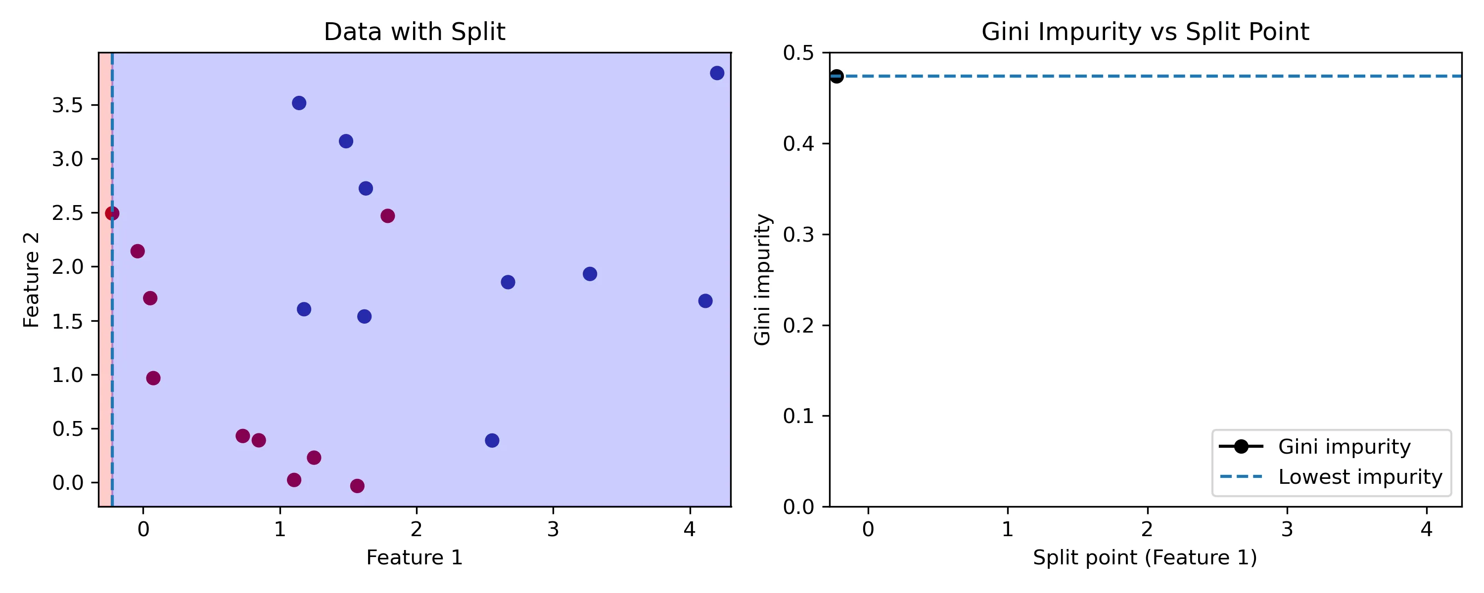
Representation of the optimization process considering a single feature. We evaluate all split points to find the one that minimizes the objective function. The same process must be done with the other features to choose the optimal split.

This approach, while computationally efficient, has significant drawbacks. The primary limitation lies in the algorithm’s inability to consider long-term consequences of split decisions. When evaluating potential splits, the algorithm optimizes only for immediate gain, potentially overlooking splits that might enable better downstream decisions.

This myopic optimization strategy introduces substantial model instability. The cumulative effect of these locally optimal but globally suboptimal decisions makes the resulting tree structure highly sensitive to variations in the training data (i.e. it’s another source of variance). In extreme cases, the addition or removal of a single training example can propagate through the tree structure, leading to dramatically different decision paths.

Moreover, this is the main reason why requiring a minimum decrease in loss to split the node is not a good idea. Splits that appear marginally beneficial in isolation may be essential for accessing valuable partition patterns deeper in the tree structure. Therefore, the immediate magnitude of improvement from a split may not reliably indicate its ultimate contribution to model performance.

Characteristics of decision trees

Assumptions

Every machine learning algorithm makes assumptions about the structure of the data. Exploring the entire space of possible relationships between features and the outcome is not feasible, therefore each algorithm cuts corners in its way.

Decision trees assume that we can separate the data into meaningful regions by repeatedly splitting on individual features. In other words, they assume that the optimal decision boundary in the feature space is axis-aligned, hence feature interactions can only be captured through hierarchical structure. As with most machine learning algorithms, these assumptions are seldom strictly true. Nonetheless, they may be close enough to reality to produce good results.

Decision trees, on the other hand, don’t make other restrictive assumptions common to many machine learning algorithms: they do not assume any probability distribution nor any linear structure. They also do not rely on any distance metric, partially evading the curse of dimensionality⁶. Feature selection is baked into the decision tree algorithm, so they can ignore irrelevant dimensions. Still, as dimensionality grows and the data becomes sparse, it becomes harder to find meaningful splits without capturing noise.

Pros and cons

We can summarize the main advantages of decision trees as:

Simple to understand and to interpret
Scales reasonably well with large datasets
Requires little data preparation⁷
Able to handle both numerical and categorical data directly
Able to approximate non-linear relationships
Do not assume any specific distribution for the data

They also same major drawbacks, namely:

Easily capture noise and overfit
Instability: highly sensitive to small changes in the training set
Lack of smooth decision boundary
Lack of smooth and continuous predictions in regression
Struggle to capture non-hierarchical concepts

Extrapolation

Decision trees do not extrapolate. I didn’t place this either as a pro or a con because it might be both.

The decision tree training procedure partitions the feature space based on examples. When a decision tree encounters a data point where one or more feature fall outside the bounds of what it was trained on, it simply assigns the value of the nearest leaf node. Therefore, predictions remain constant beyond the boundaries of the training data.

This behavior makes the model robust to extreme feature values, hence it might be desirable in some settings. However, it’s also a major limitation in domains where we expect trends to extend beyond our observed data range. Consider the task of predicting house based on constructed area. If the training data only includes houses up to 250 square meters, that is the upper bound of our predictions, even though we would reasonably expect larger houses to be more expensive. This is an inherent inductive bias of decision trees.

We’ve defined decision trees, their objective functions and a general algorithm. In the followup of this series we’ll implement classification and regression trees (CART) in Python.

References

Bias variance tradeoff - Wikipedia
Bias-Variance Analysis: Theory and Practice - Stanford CS229 (Summer 2019) lecture notes
Machine Learning for Intelligent Systems - Cornell CS4780 (Fall 2018) by Kilian Weinberger
Scikit-learn documentation on trees
Decision tree learning - Wikipedia
Machine Learning - UW-Madison STAT 479 (Fall 2018) by Sebastian Raschka
- Overview
- Decision trees lecture notes
From Theory to Practice: Inductive Biases in Machine Learning - Mindful Modeler
C. Bishop, Pattern Recognition and Machine Learning. Springer New York, 2016.
K. Murphy, Machine Learning: A Probabilistic Perspective. MIT Press, 2012.
Hastie, T., Tibshirani, R., & Friedman, J. (2009). The Elements of Statistical Learning: Data Mining, Inference, and Prediction, Second Edition. Springer New York.
Breiman, L., Friedman, J., Stone, C., & Olshen, R. (1984). Classification and Regression Trees. Taylor & Francis.
Concave function - Wikipedia
Curse of dimensionality - Wikipedia
Data processing inequality - Wikipedia
Logistic regression - Wikipedia
NP-completeness
Piecewise function - Wikipedia
Time complexity - Wikipedia

The error may not reach zero if and only if there are two or more points with exactly the same feature values but different target values. ↩
Each class was sampled from a Bivariate (2D) Gaussian distribution with SD=1. One class is shifted by 1.5 units both up and to the right. ↩
I’ve seen the term “staircase” being used informally (e.g. here) before. ↩
Not to be confused with the Gini coefficient ↩
Here, again, this split doesn’t exist only if all points have the exact same feature values. ↩
As the number of dimensions increase, the data quickly becomes sparse. Standard distance metrics (e.g. Euclidean distance) become less meaningful and loose predictive power. ↩
Decision trees are not influenced by the relative scale of features. ↩

Climbing trees 1: what are decision trees?

What is a de­ci­sion tree?

Types of trees

De­ci­sion tree al­go­rithms

Math­e­mat­i­cal de­f­i­n­i­tion

Bias-​variance trade­off

De­ci­sion tree vari­ance

De­ci­sion tree bias

The stair­case ef­fect

Ob­jec­tive func­tions

Mis­clas­si­fi­ca­tion rate

Gini im­pu­rity

En­tropy

Com­par­ing clas­si­fi­ca­tion ob­jec­tives