
Survival analysis with Cox reggression - heart failure data
Last time, we used decision trees, binarization and logistic regression to predict heart failure mortality in a public dataset. This approach yielded a very simple and parsimonious model, which, when dealing with noisy biological data and not many observations, is crucial to improve generalization.
The original data is described in this paper. As we’ve discussed previously, the time variable refers to follow-up time, that is, for how long each patient was observed. Whenever a patient that has not died reaches its follow-up time, it’s no longer observed and thus is a censored observation.
Machine learning approaches applied to this dataset generally ignore the censoring problem, which can seriously distort the results. In our previous post, we used a gimmick of filtering observations to mitigate this issue.
Nonetheless, survival analysis is the most appropriate method to analyse this dataset, as it was used in the original study. So, let’s build some survival curves and then a predictive model based on survival probability.
Let’s load the data just like last time.
library(tidyverse)
library(magrittr)
library(survival)
library(ggfortify)
library(gridExtra)
library(survminer)
library(knitr)
library(ranger)
library(riskRegression)

data <- read.csv("./heart_failure_clinical_records_dataset.csv")
factor_cols <- c("anaemia", "diabetes", "high_blood_pressure", "smoking")

data %<>% mutate_at(factor_cols, factor)
data$sex <- factor(data$sex, labels = c("female", "male"))
Using the ‘survival’ package, we’ll build a survival object and plot a survival curve:
surv_obj <- with(data, Surv(time, DEATH_EVENT))
surv_fit <- survfit(surv_obj ~ 1, data = data)

autoplot(surv_fit) + ylab("Survival Probability") + xlab("Time (days)") + theme_bw()
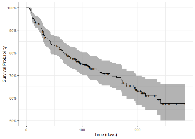
By the end of the study, only 55-60% of patients were still alive. Each + sign represents a censoring, that is, the end of one patient’s follow-up period. Let’s plot survival curves splitting by different variables:
p_anaemia <- autoplot(survfit(surv_obj ~ anaemia, data = data)) + ylab("Survival Probability") + xlab("Time (days)") + theme_bw() + theme(legend.position = "none") + ggtitle("Anaemia") + theme(plot.title = element_text(hjust = 0.5))

p_diabetes <- autoplot(survfit(surv_obj ~ diabetes, data = data)) + ylab("Survival Probability") + xlab("Time (days)") + theme_bw() + theme(legend.position = "none") + ggtitle("Diabetes") + theme(plot.title = element_text(hjust = 0.5))

p_pressure <- autoplot(survfit(surv_obj ~ high_blood_pressure, data = data)) + ylab("Survival Probability") + xlab("Time (days)") + theme_bw() + theme(legend.position = "none") + ggtitle("High blood pressure") + theme(plot.title = element_text(hjust = 0.5))

p_sex <- autoplot(survfit(surv_obj ~ sex, data = data)) + ylab("Survival Probability") + xlab("Time (days)") + theme_bw() + theme(legend.position = "none") + ggtitle("Sex") + theme(plot.title = element_text(hjust = 0.5))

p_smoking <- autoplot(survfit(surv_obj ~ smoking, data = data)) + ylab("Survival Probability") + xlab("Time (days)") + theme_bw() + theme(legend.position = "none") + ggtitle("Smoking") + theme(plot.title = element_text(hjust = 0.5))


grid.arrange(p_anaemia, p_diabetes, p_pressure, p_sex, p_smoking, nrow = 3)
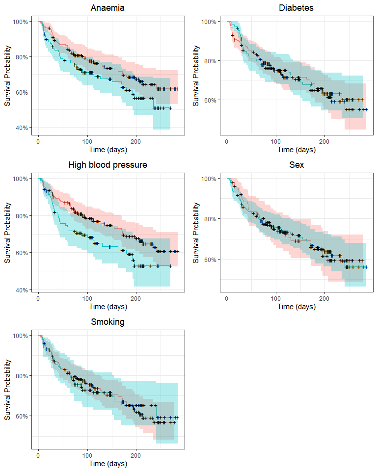
Survival may differ only by anaemia and high blood pressure status. We’ll use the log-rank test to compare survival distributions:
survdiff(surv_obj ~ data$anaemia)
## Call:
## survdiff(formula = surv_obj ~ data$anaemia)
##
##                  N Observed Expected (O-E)^2/E (O-E)^2/V
## data$anaemia=0 170       50     57.9      1.07      2.73
## data$anaemia=1 129       46     38.1      1.63      2.73
##
##  Chisq= 2.7  on 1 degrees of freedom, p= 0.1
survdiff(surv_obj ~ data$high_blood_pressure)
## Call:
## survdiff(formula = surv_obj ~ data$high_blood_pressure)
##
##                              N Observed Expected (O-E)^2/E (O-E)^2/V
## data$high_blood_pressure=0 194       57     66.4      1.34      4.41
## data$high_blood_pressure=1 105       39     29.6      3.00      4.41
##
##  Chisq= 4.4  on 1 degrees of freedom, p= 0.04
Survival distribution only differs significantly according to high blood pressure status. However, we’ve only looked at categorical variables. In fact, survival plots are not convenient to visualize the effect of continuous variables on survival. In order to explore these variables, we’ll turn them into categorical ones splitting them by their median value:
# Binning using the ntile function from dplyr
# ntile(data$serum_creatinine, 2) generates a new factor variable with
# two levels, that is, two 50th quantiles

p_age <- autoplot(survfit(surv_obj ~ ntile(log(data$age), 2), data = data)) + ylab("Survival Probability") + xlab("Time (days)") + theme_bw() + theme(legend.position = "none") + ggtitle("Age") + theme(plot.title = element_text(hjust = 0.5))

p_cpk <- autoplot(survfit(surv_obj ~ ntile(log(data$creatinine_phosphokinase), 2), data = data)) + ylab("Survival Probability") + xlab("Time (days)") + theme_bw() + theme(legend.position = "none") + ggtitle("CPK") + theme(plot.title = element_text(hjust = 0.5))

p_ef <- autoplot(survfit(surv_obj ~ ntile(log(data$ejection_fraction), 2), data = data)) + ylab("Survival Probability") + xlab("Time (days)") + theme_bw() + theme(legend.position = "none") + ggtitle("Ejection fraction") + theme(plot.title = element_text(hjust = 0.5))

p_platelets <- autoplot(survfit(surv_obj ~ ntile(log(data$platelets), 2), data = data)) + ylab("Survival Probability") + xlab("Time (days)") + theme_bw() + theme(legend.position = "none") + ggtitle("Platelets") + theme(plot.title = element_text(hjust = 0.5))

p_creatinine <- autoplot(survfit(surv_obj ~ ntile(log(data$serum_creatinine), 2), data = data)) + ylab("Survival Probability") + xlab("Time (days)") + theme_bw() + theme(legend.position = "none") + ggtitle("Serum creatinine") + theme(plot.title = element_text(hjust = 0.5))

p_sodium <- autoplot(survfit(surv_obj ~ ntile(log(data$serum_sodium), 2), data = data)) + ylab("Survival Probability") + xlab("Time (days)") + theme_bw() + theme(legend.position = "none") + ggtitle("Serum sodium") + theme(plot.title = element_text(hjust = 0.5))

grid.arrange(p_age, p_cpk, p_ef, p_platelets, p_creatinine, p_sodium, nrow = 3)
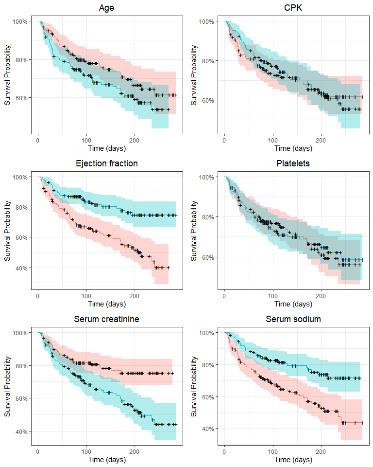
Here, ejection fraction, serum creatinine, serum sodium and (perhaps) age quantiles appear to be associated with a difference in survival. We could (and in fact I did) apply log-rank tests here, but we’ll use these variables without binning in a Cox regression. All these plots are exploratory, that is, they allow us to grasp the general tendencies and possible associations between variables. Still, they should be taken with a grain of salt because variables may have interactions and significant effects may be hidden when we split the survival curve by one variable at a time.
Cox reggression
This kind of model accepts categorical and continuous variables as predictors and estimates hazard ratios, that is, relative risks compared to a reference factor level or numerical value. It is widely use in survival analysis as it can take as input a survival curve - a very peculiar type of data. Fitting survival data with normal linear models is troublesome (among other reasons) due to high censoring frequency (inherent to survival studies). Let’s fit a simple model:
cox_m <- coxph(Surv(time, DEATH_EVENT) ~ age + anaemia + creatinine_phosphokinase + diabetes + ejection_fraction + high_blood_pressure + platelets + serum_creatinine + serum_sodium + sex + smoking, data = data, x = TRUE)

broom::tidy(cox_m) %>% kable()
| term | estimate | std.error | statistic | p.value |
|---|---|---|---|---|
| age | 0.0464082 | 0.0093240 | 4.9772722 | 0.0000006 |
| anaemia1 | 0.4601347 | 0.2168366 | 2.1220349 | 0.0338348 |
| creatinine_phosphokinase | 0.0002207 | 0.0000992 | 2.2254993 | 0.0260477 |
| diabetes1 | 0.1398841 | 0.2231472 | 0.6268692 | 0.5307450 |
| ejection_fraction | -0.0489417 | 0.0104758 | -4.6718816 | 0.0000030 |
| high_blood_pressure1 | 0.4757489 | 0.2161970 | 2.2005342 | 0.0277690 |
| platelets | -0.0000005 | 0.0000011 | -0.4115932 | 0.6806376 |
| serum_creatinine | 0.3210324 | 0.0701701 | 4.5750627 | 0.0000048 |
| serum_sodium | -0.0441875 | 0.0232657 | -1.8992585 | 0.0575305 |
| sexmale | -0.2375215 | 0.2516090 | -0.9440101 | 0.3451645 |
| smoking1 | 0.1289221 | 0.2512236 | 0.5131767 | 0.6078277 |
There are 6 significant predictors. Adding more variables will always reduce the error of a linear model. However, variables with little predictive power are most likely just adding noise to the model, and the reduced error comes from modeling random error, that is, overfitting. Just like last time, we shall keep this model simple. This is even more important considering the nature of the dataset, that is, biological data from humans, which is very noisy. There are only 96 death events, so including too many variables might quickly result in overfitting.
Thus, let’s reduce the model removing the variables which contribute very little to the final model above.
cox_m_reduced <- coxph(Surv(time, DEATH_EVENT) ~ age + anaemia + creatinine_phosphokinase + ejection_fraction + high_blood_pressure + serum_creatinine, data = data, x = TRUE)

broom::tidy(cox_m_reduced) %>% kable
| term | estimate | std.error | statistic | p.value |
|---|---|---|---|---|
| age | 0.0436066 | 0.0088530 | 4.925644 | 0.0000008 |
| anaemia1 | 0.3932590 | 0.2129360 | 1.846841 | 0.0647701 |
| creatinine_phosphokinase | 0.0001965 | 0.0000986 | 1.993298 | 0.0462289 |
| ejection_fraction | -0.0517851 | 0.0100508 | -5.152359 | 0.0000003 |
| high_blood_pressure1 | 0.4667524 | 0.2129496 | 2.191844 | 0.0283908 |
| serum_creatinine | 0.3483455 | 0.0654972 | 5.318477 | 0.0000001 |
So far so good, or is it? The cox regression model, like all models, makes a few assumptions. We’ll check for proportional hazards, influential observations and linearity in the covariates.
Cox regression models are also called proportional hazards models. This means that these models assume that the effect of a covariate is constant throughout the time, that is, residuals are independent of time. We can check this using the cox.zph function from the Survival package and by graphically inspecting if Schoenfeld residuals are independent of time.
print(cox.zph(cox_m))
##                             chisq df    p
## age                      1.03e-01  1 0.75
## anaemia                  1.69e-02  1 0.90
## creatinine_phosphokinase 1.02e+00  1 0.31
## diabetes                 1.92e-01  1 0.66
## ejection_fraction        4.69e+00  1 0.03
## high_blood_pressure      8.23e-03  1 0.93
## platelets                5.69e-06  1 1.00
## serum_creatinine         1.52e+00  1 0.22
## serum_sodium             1.10e-01  1 0.74
## sex                      7.63e-02  1 0.78
## smoking                  4.79e-01  1 0.49
## GLOBAL                   1.17e+01 11 0.39
It seems that ejection fraction does not follow the proportional hazards assumption. Still, let’s check the other assumptions and we’ll later come back to this issue. Using functions from the survminer package, let’s check for influential observations and non-linearity in the covariates.
First, let’s plot the estimated change in coefficients when each observation is removed from the model.
ggcoxdiagnostics(cox_m, type = 'dfbeta')
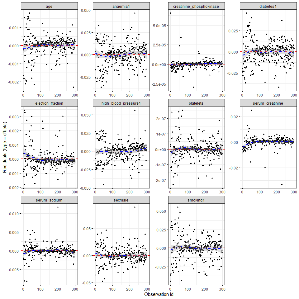
It seems that creatinine_phosphokinase, serum_creatinine and maybe serum_sodium have a few very influential observations. Finally, continuous covariate effects are assumed to be linear. We can check this assumption plotting Martingale residuals using the ggcoxfunctional function from the survminer package:
ggcoxfunctional(with(data, Surv(time, DEATH_EVENT)) ~ age + creatinine_phosphokinase + ejection_fraction + serum_creatinine + serum_sodium, data = data, ylim = c(-1, 1))
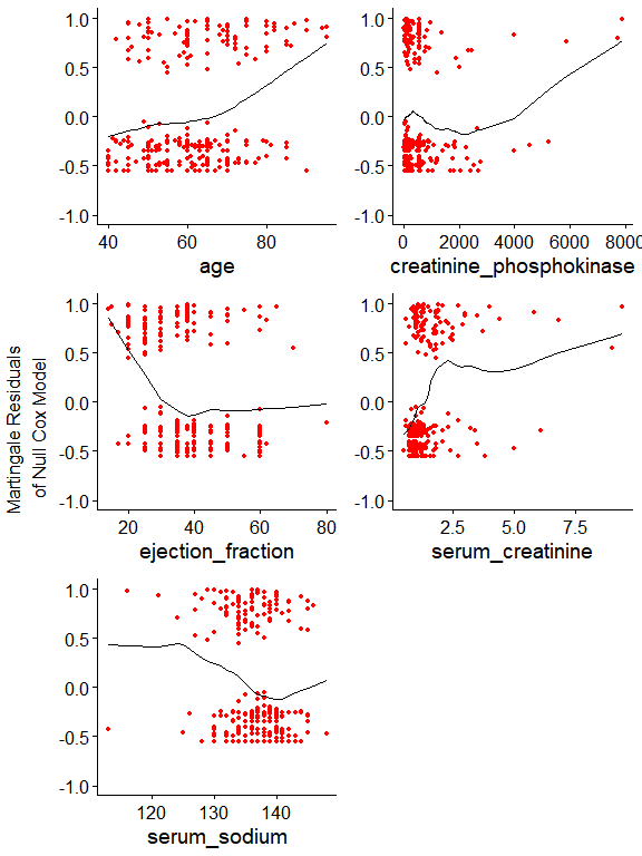
Now it’s clear why there are very influential observations. As the model assumer linear covariate effects, extremely high creatinine_phosphokinase and serum_creatinine values become largely influential. In the previous post we used binning, thus this issue became irrelevant. Here, we can address right-skewed distributions by using a simple log. The slight lef-skewed distribution of serum_sodium might not be a problem. We’ll see.
Let’s fit a new model using some log-transformed variables:
cox_m_log <- coxph(Surv(time, DEATH_EVENT) ~ age + anaemia + log(creatinine_phosphokinase) + diabetes + ejection_fraction + high_blood_pressure + platelets + log(serum_creatinine) + serum_sodium + sex + smoking, data = data, x = TRUE)

broom::tidy(cox_m_log) %>% kable()
| term | estimate | std.error | statistic | p.value |
|---|---|---|---|---|
| age | 0.0432860 | 0.0095858 | 4.5156267 | 0.0000063 |
| anaemia1 | 0.4669577 | 0.2125600 | 2.1968271 | 0.0280328 |
| log(creatinine_phosphokinase) | 0.0903269 | 0.0985837 | 0.9162459 | 0.3595379 |
| diabetes1 | 0.1435858 | 0.2228758 | 0.6442412 | 0.5194190 |
| ejection_fraction | -0.0423956 | 0.0102621 | -4.1312580 | 0.0000361 |
| high_blood_pressure1 | 0.5045094 | 0.2143303 | 2.3538880 | 0.0185782 |
| platelets | -0.0000004 | 0.0000011 | -0.3865251 | 0.6991078 |
| log(serum_creatinine) | 0.9631057 | 0.2068949 | 4.6550491 | 0.0000032 |
| serum_sodium | -0.0330688 | 0.0234632 | -1.4093885 | 0.1587203 |
| sexmale | -0.2644189 | 0.2517665 | -1.0502547 | 0.2936010 |
| smoking1 | 0.2084635 | 0.2522676 | 0.8263587 | 0.4086007 |
Interestingly, the log-transformed creatinine_phosphokinase variable was no longer a significant predictor. It looks like the fitted coefficient was largely due to extreme observations. Although omitted here, variables which contribute the least to the final model were removed in a stepwise manner, reulting in the following model:
cox_m_log <- coxph(Surv(time, DEATH_EVENT) ~ age + anaemia + ejection_fraction + high_blood_pressure + log(serum_creatinine), data = data, x = TRUE)

broom::tidy(cox_m_log) %>% kable()
| term | estimate | std.error | statistic | p.value |
|---|---|---|---|---|
| age | 0.0400060 | 0.0091061 | 4.393341 | 0.0000112 |
| anaemia1 | 0.3990274 | 0.2082361 | 1.916227 | 0.0553363 |
| ejection_fraction | -0.0443934 | 0.0099631 | -4.455787 | 0.0000084 |
| high_blood_pressure1 | 0.5084589 | 0.2112862 | 2.406494 | 0.0161065 |
| log(serum_creatinine) | 0.9932881 | 0.1892890 | 5.247469 | 0.0000002 |
The non-proportional hazard issue, however, persists:
cox.zph(cox_m_log)
##                         chisq df    p
## age                   0.17720  1 0.67
## anaemia               0.00755  1 0.93
## ejection_fraction     4.73124  1 0.03
## high_blood_pressure   0.02384  1 0.88
## log(serum_creatinine) 2.11537  1 0.15
## GLOBAL                6.65288  5 0.25
plot(cox.zph(cox_m_log)[3])
abline(c(0,0), col = 2)
abline(h = cox_m_log$coefficients[3], col = 3, lty = 2)
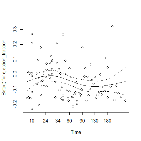
In the plot above, the green dotted line is at the fitted coefficient fot ejection_fraction. Althoug ejection fraction is a very important predictor, its effect is not constant over time. Early on it has a small negative effect on survival (close to 0 on the graph), but after 60 days its effect is much more pronounced. This is why this predictor violates the proportional hazards assumption.
A possible solution is to fit different coefficients over different time intervals (as described in this excellent vignette). Visually, it seems that splitting the data at day 50 provide a good separation of distinct ejection_fraction effects.
data_split <- survSplit(Surv(time, DEATH_EVENT) ~ ., data = data, cut = 50, episode = "tgroup", id = "id")

cox_m_split <- coxph(Surv(tstart, time, DEATH_EVENT) ~ age + anaemia + ejection_fraction:strata(tgroup) + high_blood_pressure + log(serum_creatinine), data = data_split, x = TRUE)

broom::tidy(cox_m_split) %>% kable()
| term | estimate | std.error | statistic | p.value |
|---|---|---|---|---|
| age | 0.0416812 | 0.0091931 | 4.533939 | 0.0000058 |
| anaemia1 | 0.4445463 | 0.2098468 | 2.118433 | 0.0341384 |
| high_blood_pressure1 | 0.5382776 | 0.2117104 | 2.542519 | 0.0110057 |
| log(serum_creatinine) | 0.9723897 | 0.1895731 | 5.129364 | 0.0000003 |
| ejection_fraction:strata(tgroup)tgroup=1 | -0.0189745 | 0.0118908 | -1.595734 | 0.1105482 |
| ejection_fraction:strata(tgroup)tgroup=2 | -0.0869077 | 0.0176826 | -4.914874 | 0.0000009 |
The ejection fraction now only has a significant effect on tgroup = 2, that is, after day 50. This should remove the issue with the non-proportional hazard. Let’s check:
print(cox.zph(cox_m_split))
##                                    chisq df    p
## age                              0.02004  1 0.89
## anaemia                          0.15881  1 0.69
## high_blood_pressure              0.00366  1 0.95
## log(serum_creatinine)            1.35157  1 0.25
## ejection_fraction:strata(tgroup) 1.13453  2 0.57
## GLOBAL                           3.14512  6 0.79
Great! The assumption is not violated anymore. Now we’ll compare the models we have built so far. For this step, we’ll split the data into training (70% of original data) and test (30%) datasets and refit the previous models using the training data.
set.seed(12)
train_size = floor(0.7 * nrow(data))
train_ind <- sample(seq_len(nrow(data)), size = train_size)

train_data <- data[train_ind, ]
test_data <- data[-train_ind, ]

cox_m_log <- coxph(Surv(time, DEATH_EVENT) ~ age + anaemia + log(creatinine_phosphokinase) + diabetes + ejection_fraction + high_blood_pressure + platelets + log(serum_creatinine) + serum_sodium + sex + smoking, data = train_data, x = TRUE)
cox_m_log_reduced <- coxph(Surv(time, DEATH_EVENT) ~ age + anaemia + ejection_fraction + high_blood_pressure + log(serum_creatinine), data = train_data, x = TRUE)

train_data_split <- survSplit(Surv(time, DEATH_EVENT) ~ ., data = train_data, cut = 50, episode = "tgroup", id = "id")

cox_m_split <- coxph(Surv(tstart, time, DEATH_EVENT) ~ age + anaemia + ejection_fraction:strata(tgroup) + high_blood_pressure + log(serum_creatinine), data = train_data_split, x = TRUE)


models = list(cox_m_log, cox_m_log_reduced, cox_m_split)
concordances = sapply(models, function(x) concordance(x)$concordance)
aics = sapply(models, AIC)

models_metrics = data.frame(Model = c('All variables', 'Selected variables', 'Split time, selected var.'), Concordance = concordances, AIC = aics)
models_metrics %>% kable()
| Model | Concordance | AIC |
|---|---|---|
| All variables | 0.7458686 | 606.5232 |
| Selected variables | 0.7391677 | 599.1368 |
| Split time, selected var. | 0.7455159 | 593.9153 |
Our final model, which doesn’t violate the core model assumptions, presents better AIC compared to the previous ones and a very similar concordance compared to the model with all variables. But in practice this model will predict two separate survival curves, one for each tgroup (before or after day 50). Therefore, this model may be great to interpret the contribution of each variable, but it’s not very practical for prediction.
Finally, we’ll build a random survival forest model using the ranger function from the ranger package. However, we’ll not go deep into this model. We’ll limit tree depth (max.depth) and set a higher minimal node size (min.node.size) to avoid overfitting.
ranger_m <- ranger(Surv(time, DEATH_EVENT) ~ age + anaemia + creatinine_phosphokinase + diabetes + ejection_fraction + high_blood_pressure + platelets + serum_creatinine + serum_sodium + sex + smoking, data = train_data, x = TRUE, importance = 'permutation', min.node.size = 5, max.depth = 5)
The riskRegression package has a nice Score function that calculates Brier scores and Index of Prediction Accuracy, which is 1 minus the ratio between the Brier score of the model against the Brier score of a null model. A positive IPA means a better probability prediction compared to the null model.
ipa_models <- Score(list("Cox - all variables" = cox_m_log, "Cox - few variables" = cox_m_log_reduced, "Reduced" = ranger_m), data = test_data, formula = Surv(time, DEATH_EVENT) ~ 1, summary = 'ipa', metrics = 'brier', contrasts = FALSE)

print(ipa_models)
##
## Metric Brier:
##
## Results by model:
##
##                  model times Brier lower upper  IPA
## 1:          Null model   113  20.9  15.8  26.0  0.0
## 2: Cox - all variables   113  16.3  10.4  22.2 21.9
## 3: Cox - few variables   113  15.8  10.0  21.6 24.3
## 4:             Reduced   113  16.4  11.7  21.2 21.3

##
## NOTE: Values are multiplied by 100 and given in %.

## NOTE: The lower Brier the better, the higher IPA the better.
It seems our Cox regression with only a few variables outperforms the other models slightly (higher IPA score). Random forests can be really useful to fit high dimensional data. In this case, however, a Cox regression carefully fit seems to be an excellent option.
Leave a comment