
Warning: this post talks about suicide and should be read with caution.
The Data
Exploratory data analysis is essential to construct hypothesis. Today we’ll explore the publicly available WHO Suicide Statistics database (version from Kaggle). It consists of a single CSV table, with 43776 instances of merely 6 variables. We do not intend to speculate about suicide causes nor to make any judgements. This analysis was done using R and R markdown.
summary(who_suicide_statistics)
##    country               year          sex                age
##  Length:43776       Min.   :1979   Length:43776       Length:43776
##  Class :character   1st Qu.:1990   Class :character   Class :character
##  Mode  :character   Median :1999   Mode  :character   Mode  :character
##                     Mean   :1999
##                     3rd Qu.:2007
##                     Max.   :2016
##
##   suicides_no        population
##  Min.   :    0.0   Min.   :     259
##  1st Qu.:    1.0   1st Qu.:   85113
##  Median :   14.0   Median :  380655
##  Mean   :  193.3   Mean   : 1664091
##  3rd Qu.:   91.0   3rd Qu.: 1305698
##  Max.   :22338.0   Max.   :43805214
##  NA's   :2256      NA's   :5460
Clearly, we have a considerable amount of missing values, with data since 1979 to 2016, which is still quite recent. The sex and country variables must be converted to categorical ones:
who_suicide_statistics$sex <- as.factor(who_suicide_statistics$sex)
who_suicide_statistics$country <- as.factor(who_suicide_statistics$country)
Next, the age variable should be an ordered factor:
who_suicide_statistics$age <- factor(who_suicide_statistics$age, levels = c("5-14 years", "15-24 years", "25-34 years", "55-74 years", "75+ years"))
Let’s take a look at our most important variable – suicide number:
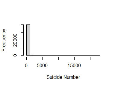
Clearly, the distribution is extremely skewed and zero-inflated, ranging from 0 to very high values. Let’s create a proportional suicide number variable (suicide_rate), defined by prop_suicide = suicides_no/population * 1000000 (per million people) and see its distribution:
total_suicide_rate <- who_suicide_statistics %>% group_by(country, year) %>% summarise(rate_suicide = sum(suicides_no) * 1000000 / sum(population), .groups = "drop_last") %>% na.omit

hist(total_suicide_rate$rate_suicide, xlab = "Suicide rate", main = NA)
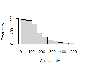
Much less variance, but still a very broad range. Let’s summarise and plot some graphs to see the relationships between variables.
library(ggplot2, dplyr)
## Warning: package 'ggplot2' was built under R version 4.0.5
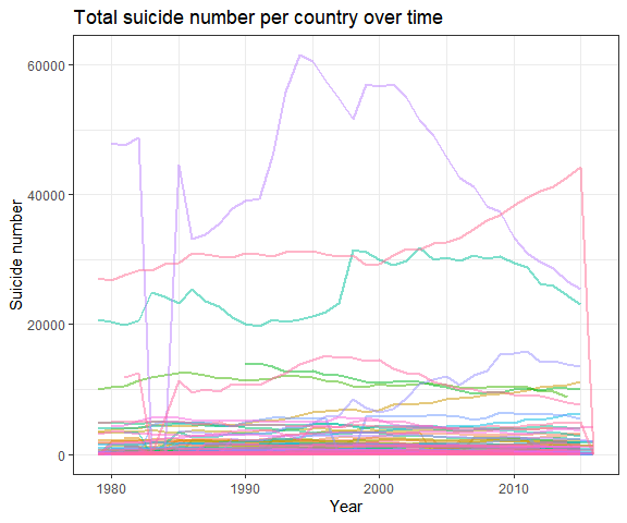
total_suicide <- who_suicide_statistics %>% group_by(year, country) %>% summarise(total_suicide = sum(suicides_no, na.rm = T), .groups = "drop_last")
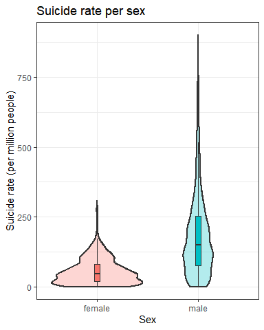
Men have higher suicide rates overall Let’s see which countries have the most and least suicides:
Top 10 countries and correspondent years with highest suicide rates
| country | year | rate_suicide |
|---|---|---|
| Lithuania | 1996 | 510.1976 |
| Lithuania | 1995 | 500.1256 |
| Lithuania | 1994 | 499.8927 |
| Hungary | 1983 | 492.1207 |
| Lithuania | 2000 | 491.9875 |
| Hungary | 1981 | 491.5882 |
| Hungary | 1984 | 490.6624 |
| Hungary | 1980 | 486.1906 |
| Lithuania | 1997 | 485.0974 |
| Hungary | 1979 | 485.0378 |
Top 10 countries and correspondent years with lowest positive suicide rates
| country | year | rate_suicide |
|---|---|---|
| Egypt | 1980 | 0.4035020 |
| Jamaica | 2004 | 0.4057770 |
| Jamaica | 1991 | 0.4640727 |
| Jamaica | 1986 | 0.4872034 |
| Egypt | 2007 | 0.4927728 |
| Egypt | 1987 | 0.4942756 |
| Jamaica | 1982 | 0.5138543 |
| Egypt | 2002 | 0.5620709 |
| Egypt | 2015 | 0.6084794 |
| Egypt | 2008 | 0.6107135 |
Now let’s take an average over the last five years of data and see again the highs and lows:
Top 20 countries with highest suicide rates (2012-2016 average)
| country | rate_suicide |
|---|---|
| Lithuania | 335.3883 |
| Guyana | 305.1528 |
| Republic of Korea | 289.2143 |
| Suriname | 265.4565 |
| Slovenia | 217.4291 |
| Hungary | 212.4062 |
| Latvia | 209.5409 |
| Kazakhstan | 208.0467 |
| Japan | 207.0399 |
| Belarus | 204.4635 |
| Russian Federation | 203.9287 |
| Ukraine | 198.5692 |
| Uruguay | 186.5003 |
| Belgium | 182.3194 |
| Croatia | 179.5992 |
| Estonia | 178.9021 |
| Serbia | 169.9654 |
| Republic of Moldova | 168.2837 |
| Mongolia | 166.7801 |
| Poland | 166.0466 |
Top 20 countries with lowest positive suicide rates (2012-2016 average)
| country | rate_suicide |
|---|---|
| Egypt | 1.596867 |
| Oman | 1.927792 |
| Antigua and Barbuda | 2.720674 |
| Grenada | 4.191730 |
| Bahrain | 9.113524 |
| Mayotte | 10.501900 |
| South Africa | 11.001666 |
| Bahamas | 14.440957 |
| Kuwait | 15.263111 |
| Brunei Darussalam | 15.960329 |
| Turkey | 22.758229 |
| Qatar | 23.989111 |
| Armenia | 24.627670 |
| Venezuela (Bolivarian Republic of) | 24.873804 |
| Turkmenistan | 26.545199 |
| Iran (Islamic Rep of) | 34.028634 |
| Guatemala | 34.051098 |
| Saint Vincent and Grenadines | 37.354314 |
| Panama | 37.454562 |
| Fiji | 40.871639 |
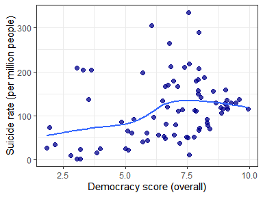
Let’s see if there’s any relationship between suicide rates (2012-2016) and Democracy Index (2015) calculated by The Economist group. The democracy index data was manually curated to correspond to country names present in the WHO dataset.
democracy <- read.csv(file = "democracy_index_2015.csv")

democracy_compare_data <- total_suicide_rate %>% filter(year >= 2012) %>% filter(country %in% as.character(unique(democracy$Country))) %>% group_by(country) %>% summarise(rate_suicide = mean(rate_suicide, na.rm = T)) %>% arrange(country)

democracy <- democracy %>% filter(Country %in% as.character(unique(democracy_compare_data$country))) %>% arrange(Country)

democracy_compare_data$overall_score <- democracy$Overall_score

ggplot(data = democracy_compare_data, aes(overall_score, rate_suicide)) + geom_point(size = 2, alpha = 0.75, colour = "dark blue") + theme_bw() + geom_smooth(formula = y ~ x, method = "loess", se = F) + xlab("Democracy score (overall)") + ylab("Suicide rate (per million people)")
tidy(cor.test(democracy$Overall_score, democracy_compare_data$rate_suicide, method = "pearson")) %>% kable()
| estimate | statistic | p.value | parameter | conf.low | conf.high | method | alternative |
|---|---|---|---|---|---|---|---|
| 0.3072375 | 2.833023 | 0.0058833 | 77 | 0.0924044 | 0.4947386 | Pearson’s product-moment correlation | two.sided |
tidy(cor.test(democracy$Overall_score, democracy_compare_data$rate_suicide, method = "spearman")) %>% kable()
| estimate | statistic | p.value | method | alternative |
|---|---|---|---|---|
| 0.3547168 | 53016.47 | 0.0013388 | Spearman’s rank correlation rho | two.sided |
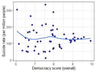
There’s a weak (R = 0.307) but significant positive Pearson correlation between the Democracy Index and suicide rates. However, there are many confounding factors here, as more democratic countries are in general richer and may report suicide statistics with better accuracy. Also, there are huge cultural differences between countries. Among highly democratic nations the correlation is near zero:
democracy_compare_data %>% filter(overall_score > 6) %>% ggplot(aes(overall_score, rate_suicide)) + geom_point(size = 2, alpha = 0.75, colour = "dark blue") + theme_bw() + geom_smooth(formula = y ~ x, method = "loess", se = F) + xlab("Democracy score (overall)") + ylab("Suicide rate (per million people)")
Gross domestic product based on purchasing-power-parity (PPP) per capita GDP values (2015) in international dollars were obtained from the International Monetary Fund (IMF).
gdppc <- read.csv("WEO_Data.xls", sep = "\t")
gdppc$X2015 <- as.numeric(as.character(gdppc$X2015))

gdp_compare_data <- total_suicide_rate %>% filter(year >= 2012) %>% filter(country %in% as.character(unique(gdppc$Country))) %>% group_by(country) %>% summarise(rate_suicide = mean(rate_suicide, na.rm = T)) %>% arrange(country)

gdppc <- gdppc %>% filter(Country %in% as.character(unique(gdp_compare_data$country))) %>% arrange(Country)
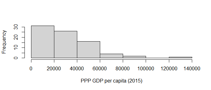
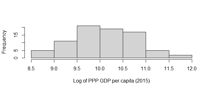
As the GDP variable is heavily skewed, it’s better to visualize it using its log transform:
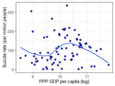
tidy(cor.test(gdppc$X2015, gdp_compare_data$rate_suicide, method = "spearman")) %>% kable()
| estimate | statistic | p.value | method | alternative |
|---|---|---|---|---|
| 0.1861228 | 69440 | 0.0983024 | Spearman’s rank correlation rho | two.sided |
There does not seem to exist an apparent association between suicide rates and per capita GDP income.
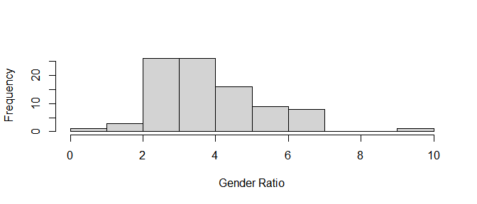
Gender Ratios
female_rates <- who_suicide_statistics %>% filter(year >= 2012) %>% group_by(country, sex) %>% summarise(rate_suicide = sum(suicides_no) * 1000000 / sum(population), .groups = "drop_last") %>% na.omit %>% arrange(country) %>% filter(sex == "female")

male_rates <- who_suicide_statistics %>% filter(year >= 2012) %>% group_by(country, sex) %>% summarise(rate_suicide = sum(suicides_no) * 1000000 / sum(population), .groups = "drop_last") %>% na.omit %>% arrange(country) %>% filter(sex == "male")

gender_ratio <- data.frame(country = female_rates$country, ratio = male_rates$rate_suicide / female_rates$rate_suicide) %>% na.omit() %>% filter(is.finite(ratio))

hist(gender_ratio$ratio, main = NA, xlab = "Gender Ratio")
gender_ratio_gdp <- gender_ratio %>% filter(country %in% as.character(unique(gdppc$Country)))
gdppc_gender <- gdppc %>% filter(Country %in% as.character(unique(gender_ratio_gdp$country)))
#ggplot(data = gender_ratio_gdp, aes(log(gdppc_gender$X2015), ratio)) + geom_point(size = 2, alpha = 0.75, colour = "dark blue") + theme_bw() + geom_smooth(se=F)

tidy(cor.test(gender_ratio_gdp$ratio, gdppc_gender$X2015)) %>% kable()
| estimate | statistic | p.value | parameter | conf.low | conf.high | method | alternative |
|---|---|---|---|---|---|---|---|
| -0.2276648 | -1.956149 | 0.0544387 | 70 | -0.4363206 | 0.0042267 | Pearson’s product-moment correlation | two.sided |
gender_ratio_dem <- gender_ratio %>% filter(country %in% as.character(unique(democracy$Country)))
democracy_gender <- democracy %>% filter(Country %in% as.character(unique(gender_ratio_dem$country)))
#ggplot(data = gender_ratio_dem, aes(democracy_gender$Overall_score, ratio)) + geom_point(size = 2, alpha = 0.75, colour = "dark blue") + theme_bw() + geom_smooth(se=F)

tidy(cor.test(gender_ratio_dem$ratio, democracy_gender$Overall_score)) %>% kable()
| estimate | statistic | p.value | parameter | conf.low | conf.high | method | alternative |
|---|---|---|---|---|---|---|---|
| -0.0795524 | -0.6724517 | 0.5034788 | 71 | -0.3040547 | 0.153321 | Pearson’s product-moment correlation | two.sided |
There does not seem to be any association between gender ratios and Democracy Index nor per capita GDP.
Top 10 countries with highest gender ratios (male-to-female) 2012-2016
head(gender_ratio %>% arrange(desc(ratio)), n = 20) %>% kable()
| country | ratio |
|---|---|
| Bahrain | 9.262603 |
| Poland | 6.992961 |
| Saint Lucia | 6.889143 |
| Seychelles | 6.841246 |
| Slovakia | 6.684513 |
| Panama | 6.439133 |
| Mongolia | 6.425235 |
| Puerto Rico | 6.290557 |
| Costa Rica | 6.000486 |
| Romania | 5.962328 |
| Republic of Moldova | 5.751732 |
| Belize | 5.586587 |
| Latvia | 5.480794 |
| Lithuania | 5.463001 |
| Russian Federation | 5.419557 |
| Cyprus | 5.224378 |
| Reunion | 5.115328 |
| Ukraine | 5.011528 |
| Malta | 4.980026 |
| Georgia | 4.875833 |
Top 10 countries with lowest positive gender ratios (male-to-female) 2012-2016
head(gender_ratio %>% filter(ratio > 0) %>% arrange(ratio), n = 20) %>% kable()
| country | ratio |
|---|---|
| Kuwait | 1.472849 |
| Aruba | 1.903816 |
| Hong Kong SAR | 1.915214 |
| Uzbekistan | 2.076370 |
| Singapore | 2.079089 |
| Iran (Islamic Rep of) | 2.116816 |
| Fiji | 2.120162 |
| Netherlands | 2.211227 |
| Republic of Korea | 2.304564 |
| Norway | 2.332093 |
| Sweden | 2.360817 |
| Japan | 2.424445 |
| Virgin Islands (USA) | 2.484681 |
| Paraguay | 2.492538 |
| Turkmenistan | 2.578286 |
| Luxembourg | 2.584304 |
| Belgium | 2.614295 |
| Guatemala | 2.636253 |
| Saint Vincent and Grenadines | 2.699769 |
| New Zealand | 2.759721 |
Age
Elderly suicide is an increasingly troublesome concern as the population grows older.
elderly_data <- who_suicide_statistics %>% filter(year >= 2012) %>% filter(age == "55-74 years" | age == "75+ years") %>% group_by(country) %>% summarise(rate_suicide = sum(suicides_no) * 1000000 / sum(population)) %>% na.omit %>% arrange(desc(rate_suicide))
Top 10 countries with highest elderly suicide rates (2012-2016)
head(elderly_data, n = 10) %>% kable()
| country | rate_suicide |
|---|---|
| Republic of Korea | 494.6145 |
| Lithuania | 391.9060 |
| Slovenia | 346.1632 |
| Hungary | 342.0108 |
| Guyana | 333.2012 |
| Suriname | 307.5963 |
| Serbia | 296.0792 |
| Croatia | 289.7782 |
| Cuba | 277.7552 |
| Uruguay | 261.7103 |
This, however, can be biased due to a higher overall higher incidence of suicides in some countries. Thus, let’s calculate the percentage of total suicides that are elderly ones (55+ years).
total_elderly <- who_suicide_statistics %>% filter(year >= 2012) %>% filter(age == "55-74 years" | age == "75+ years") %>% group_by(country) %>% summarise(total_suicide = sum(suicides_no)) %>% na.omit

total_2012_16 <- total_suicide %>% filter(year >= 2012) %>% group_by(country) %>% summarise(total_suicide = sum(total_suicide, na.rm = T)) %>% filter(country %in% as.character(unique(total_elderly$country)))

elderly_proportion <- data.frame(country = total_elderly$country, proportion = total_elderly$total_suicide / total_2012_16$total_suicide)

elderly_proportion <- elderly_proportion[is.finite(elderly_proportion$proportion), ]
Top 10 countries with highest elderly suicide proportion (2012-2016)
head(elderly_proportion %>% arrange(desc(proportion)), n = 10) %>% kable()
| country | proportion |
|---|---|
| Antigua and Barbuda | 1.0000000 |
| Serbia | 0.6119500 |
| Portugal | 0.5895522 |
| Bulgaria | 0.5839448 |
| Croatia | 0.5570321 |
| Hungary | 0.5400160 |
| Germany | 0.5384444 |
| Austria | 0.5329861 |
| Slovenia | 0.5318396 |
| Cuba | 0.5177912 |
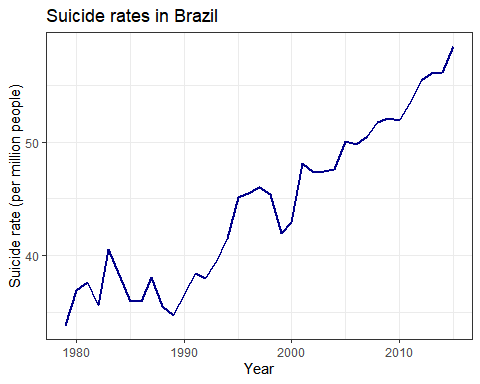
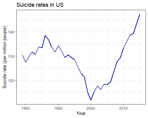
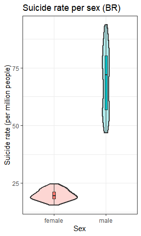
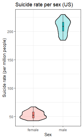
USA and Brazil: a case-study
I’ve selected two countries for further analysis: Brazil and USA, both very big countries with reliable data.
BR_data <- subset(who_suicide_statistics, country == "Brazil")

US_data <- subset(who_suicide_statistics, country == "United States of America")
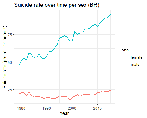
Gender differences can be calculated over time:
sex_US_data <- US_data %>% group_by(year, sex) %>% summarise(rate_suicide = sum(suicides_no) * 1000000 / sum(population), .groups = "drop_last") %>% na.omit

sex_BR_data <- BR_data %>% group_by(year, sex) %>% summarise(rate_suicide = sum(suicides_no) * 1000000 / sum(population), .groups = "drop_last") %>% na.omit

US_data_sexratio <- data.frame(year = subset(sex_US_data, sex == "male")$year, ratio = subset(sex_US_data, sex == "male")$rate_suicide / subset(sex_US_data, sex == "female")$rate_suicide, country = "US")

BR_data_sexratio <- data.frame(year = subset(sex_BR_data, sex == "male")$year, ratio = subset(sex_BR_data, sex == "male")$rate_suicide / subset(sex_BR_data, sex == "female")$rate_suicide, country = "BR")

data_sexratio <- rbind(US_data_sexratio, BR_data_sexratio)
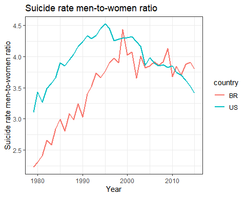
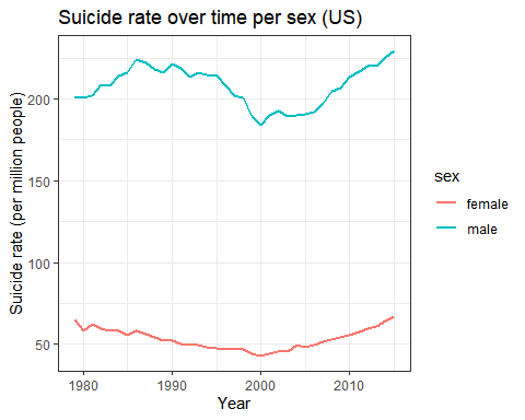
In Brazil, suicide rates for men have been steadily increasing since the 1980s, while rates for women have stayed roughly the same. In the US, however, suicide rates for men increased during the 80s (not followed by an increase in women’s rates), decline in the 2000s and has been increasing since 2005-6. This increase is now followed by a similar (but smaller) one in women’s rates. Thus, the men-to-women ratio increased with time in Brazil and decreased only after 2000 in the US. In 2015, for each woman, 4-4.5 men have ended their lives in Brazil or in the US.
age_data_usbr <- who_suicide_statistics %>% group_by(year, country, age) %>% summarise(rate_suicide = sum(suicides_no) * 1000000 / sum(population), .groups = "drop_last") %>% na.omit
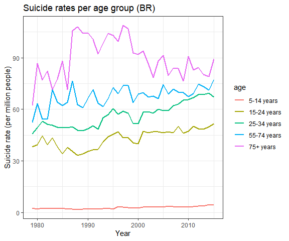
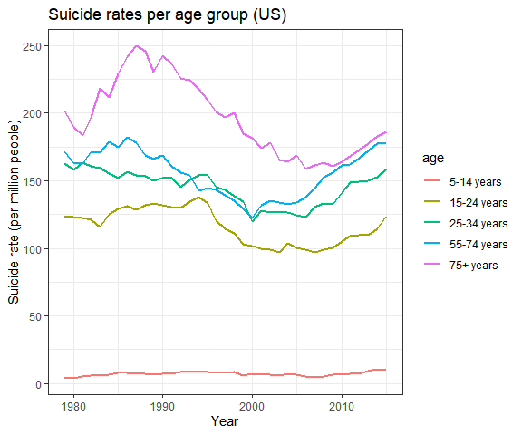
Both countries present highest suicide rates for the elderly. However, in both cases, the gap between adults (25-34 years) and elderly (55+ years) is getting narrower since the 2000s, which shows that adult suicide is more likely now than compared to the past (1990s).
age_gender_usbr <- who_suicide_statistics %>% group_by(sex, year, country, age) %>% summarise(rate_suicide = sum(suicides_no) * 1000000 / sum(population), .groups = "drop_last") %>% na.omit
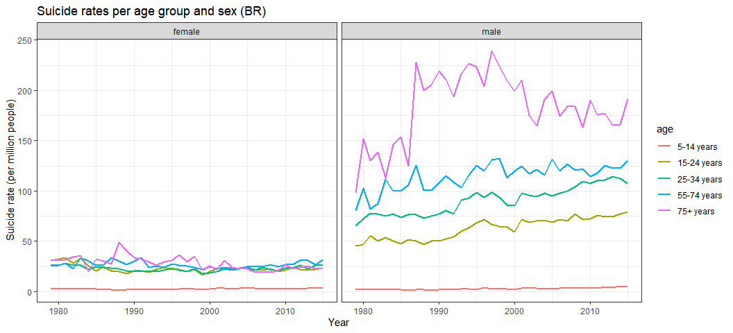
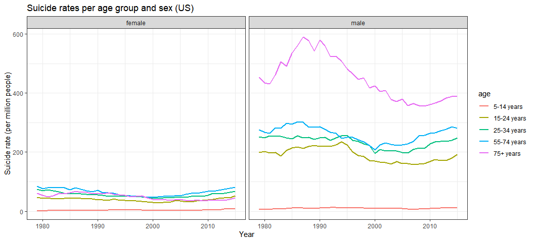
Interestingly, the high elderly suicide rate is apparently accounted for by only male people. There’s practically no age gap among women. This suggests that elderly suicide is almost exclusively a male issue in these countries.
Conclusion
This exploratory analysis is descriptive and serves the purpose to inform about overall characteristics and trends in global suicide reports provided by the WHO. Suicide is a complex social phenomenon and should not be interpreted simplistically. Still, the huge difference between genders in the age gap is of interest.
Leave a comment