The basics of outlier detection

Outliers

The word outlier is frequently used in my field of research (basic biology and biomedicine). It refers to data observations that differ a lot from the others. Some very informative posts regarding outliers are already available (see here and here for examples). However, my experience is that biology researchers often don’t receive adequate statistical education and rely on possibly dangerous heuristics to determine what is an outlier. This post is intended to explain the basics of outlier detection and removal and, more specifically, to highlight some common mistakes. Outliers may arise from experimental errors, human mistakes, flawed techniques (eg a batch of experiments done with low-quality reagent), corrupt data, or simply sampling probability.

Why do people remove outliers?

The question is valid: if data is obtained through standardized and reproducible procedures, why should valuable data points be tossed out? The answer is that standard statistical tests that rely on parametric assumptions are quite sensitive to outliers. This occurs mainly (but not exclusively) because the mean is very sensitive to extreme values (while the median is not, for example) - and the standard error is also sensitive in some way. So, as parametric tests usually rely solely on mean and variances to calculate the famous p-value, outliers often lead to weird results that do not seem plausible. For instance, let’s consider the data: 2.051501, 3.278150, 1.532082, 3.826658, 2.335235

A one-sample t-test tests if the mean is significantly different from zero. The result is that, as one would expect, it is indeed:

##
##  One Sample t-test
##
## data:  c(2.051501, 3.27815, 1.532082, 3.826658, 2.335235)
## t = 6.2481, df = 4, p-value = 0.003345
## alternative hypothesis: true mean is not equal to 0
## 95 percent confidence interval:
##  1.447266 3.762184
## sample estimates:
## mean of x
##  2.604725

However, let’s now add a point that makes the data even farther from zero: 2.051501, 3.278150, 1.532082, 3.826658, 2.335235, 20

##
##  One Sample t-test
##
## data:  c(2.051501, 3.27815, 1.532082, 3.826658, 2.335235, 20)
## t = 1.8855, df = 5, p-value = 0.118
## alternative hypothesis: true mean is not equal to 0
## 95 percent confidence interval:
##  -1.999914 13.007789
## sample estimates:
## mean of x
##  5.503938

Well, now there’s no significant difference. The standard deviation of the sample increases a lot with the artificial outlier and so does the standard error of the mean, which is used to calculate confidence intervals and p-values. Thus, back in time when parametric statistics were all that there was and sample sizes were very limited, the solution was to remove (or change the value of) the outlying values.

Now, at this point it’s important to notice a few characteristics about outliers: by definition, outliers must be rare. If outliers are common (that is, more than a few percent of the observations at most), probably some data collection error has happened or the distribution is very far from a normal one. Another option is that the outlier detection method implemented detects too much of them.

Detecting outliers

Z-scores

Z-scores are simply a way to standardize your data through rescaling. It shows how many standard deviations a given point, well, deviates from the mean. One can set an arbitrary threshold and exclude points that are above the positive threshold value or below the negative one. Let’s apply the z-score to our artificial data with a threshold value of 2:

print(scale(c(2.051501, 3.27815, 1.532082, 3.826658, 2.335235, 20))[, 1])

## [1] -0.4828334 -0.3112829 -0.5554757 -0.2345725 -0.4431524  2.0273168

This shows that our artificial outlier is indeed above the threshold and could be removed. However, many people consider 2 a far too permissive threshold and use 3 as a rule-of-thumb value. The outlier threshold will always be arbitrary and there’s no right answer, but using a low value can lead to frequent outlier detection - and outliers must be rare.

So, to sum it up, the z-score method is quite effective if the distribution of the data is roughly normal. The smaller the sample size, the more influence extreme values will have over the mean and the standard deviation. Thus, the z-score method may fail to detect extreme values in small sample sizes.

IQR method

The interquartile range (or IQR) method was created by the great statistician John Tukey and is embedded in the famous boxplot. The idea is to determine the 25th and 75th quantiles, that is, the values that leave 25% and 75% of the data below it, respectively. Then, the distance between them is the IQR. Below you can see a histogram of the famous height data from Sir Francis Galton in which those quantiles are marked with red lines. 50% of the data lies between the lines.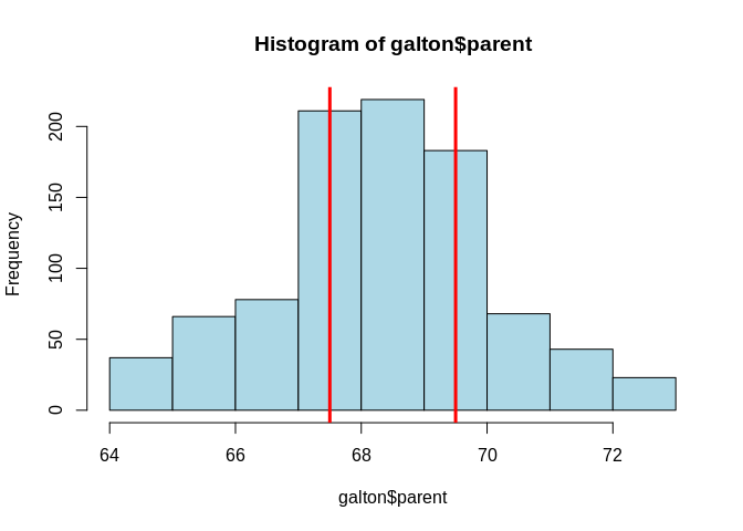

The box-and-whisker plot (or boxplot) simply draws a box whose limits are the 25th and 75th percentiles, with the median (or 50th percentile) as a line in the middle. Then, whiskers of length 1.5 times IQR are drawn on both directions, that is, 1.5 times IQR below the 25th percentile and 1.5 times IQR above the 75th percentile. Values that are outside this range were considered outliers by Tukey. Here is the boxplot for the height data: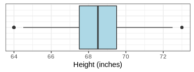

Some outliers do appear, but they are very few. The main advantage of the IQR method is that it’s more robust to slightly skewed distributions and it can detect outliers with smaller sample sizes as the median and IQR are much less influenced by extreme values than the mean and standard deviation, respectively. With z-scores, the presence of really extreme values can influence the mean and the standard deviation so much that it fails to detect other less extreme outliers, a phenomenon known as masking. In some cases, a factor of 2 or even 3 is used to multiply the IQR, detecting fewer outliers.

Using our previous artificial data, let’s replace the outlier with a less extreme value of 8 and apply both detection methods:

print(scale(c(2.051501, 3.27815, 1.532082, 3.826658, 2.335235, 8))[, 1])

## [1] -0.61670998 -0.09587028 -0.83725721  0.13702825 -0.49623548  1.90904470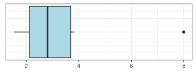

The z-score method does not detect the extreme value as an outlier, while the IQR method does so. Let’s increase the sample size and repeat the analysis. The new data will be: 2.0515010, 3.2781500, 1.5320820, 3.8266580, 2.3352350, 3.4745626, 0.3231792, 3.3983499, 2.7515991, 4.5479615, 1.3167715, 1.8196742, 2.1908817, 1.8590404, 2.6546580, 3.5424431, 2.9777304, 2.6038048, 4.5722174, 8

print(scale(c(2.0515010, 3.2781500, 1.5320820, 3.8266580, 2.3352350, 3.4745626, 0.3231792, 3.3983499, 2.7515991, 4.5479615, 1.3167715, 1.8196742, 2.1908817, 1.8590404, 2.6546580, 3.5424431, 2.9777304, 2.6038048, 4.5722174, 8))[, 1])

##  [1] -0.56445751  0.20373600 -0.88974560  0.54724118 -0.38676803
##  [6]  0.32674012 -1.64682548  0.27901164 -0.12601846  0.99896019
## [11] -1.02458460 -0.70963991 -0.47716983 -0.68498668 -0.18672819
## [16]  0.36925054  0.01559711 -0.21857520  1.01415054  3.16081217

Now the artificial value is identified as an outlier, although the average of the other points is roughly the same. That is because the standard deviation and the mean get less sensitive to extreme values as the sample size increases. The IQR method also identifies the artificial point as an outlier in this case (graph not shown). The z-score, by definition, will never be greater than (n-1)/\(\sqrt{n})\), and that should be accounted for before analysis.

MAD method

The last method that we’ll cover is based on the median absolute deviation (MAD) and this method is often referred to as the robust z-score. It’s essentially a z-score, except the median will be used instead of the mean and the MAD instead of the standard deviation. The MAD is the median of the absolute values of the distance between each point and the sample median. In other words, it’s a standard deviation calculated with medians instead of averages. The new score, let’s call it the M-score, is given by: \[M_i = \displaystyle \frac{0.6745(x_i - \tilde{x})}{MAD}\] Where \(\tilde{x}\) is the sample median and \(x_i\) is each observation. Various thresholds have been suggested, ranging between 2 and 3. Let’s apply this method to our artificial outlier of 8 with a threshold of 2.24 as suggested before (Iglewicz and Hoaglin 1993):

m_data <- c(2.051501, 3.27815, 1.532082, 3.826658, 2.335235, 8)
print(0.6745*(m_data - median(m_data)) / mad(m_data))

## [1] -0.3870867  0.2416539 -0.6533241  0.5228013 -0.2416539  2.6619214

The artificial outlier is indeed above the threshold. The M-score suffers even less masking than the IQR and much less than the z-score. It’s robust to extreme outliers even with small sample sizes.

The dangers of outlier removal

False positives (type I error)

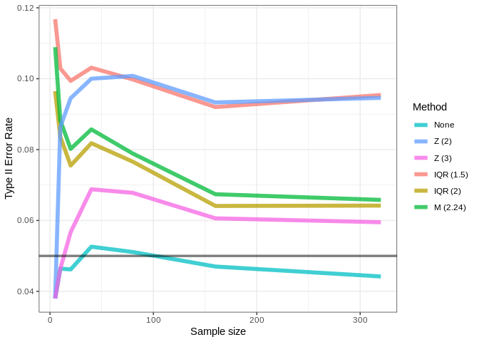
When performing exploratory data analysis, all outlier detection methods listed above are valid and each one has its pros and cons. They are useful to detect possible flaws in data collection but are also very useful to detect novelty and new trends. However, when performing inferential analysis, type I error rates (false positives) should be accounted for. Here, we’ll accept a 5% type I error rate, as usual. The graphic below shows the type I error rate for a two-sample Welch t-test drawing samples from a population of 10000 normally distributed points (mean = 0, sd = 1). For each sample sizes, 10000 t-tests are performed on independent samples.

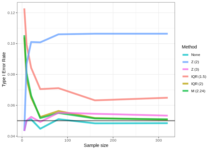
It’s quite alarming that, when using a threshold of \(|Z-score|\) > 2, the error rate goes up as the sample size increases. This shows that, although this is a very common threshold in published studies, it greatly inflates error rates and can be considered a form of p-hacking. All methods resulted in error inflation, especially with smaller sample sizes. Let’s repeat this analysis using a population with skewed values:

population <- rgamma(10000, shape = 6)
hist(population)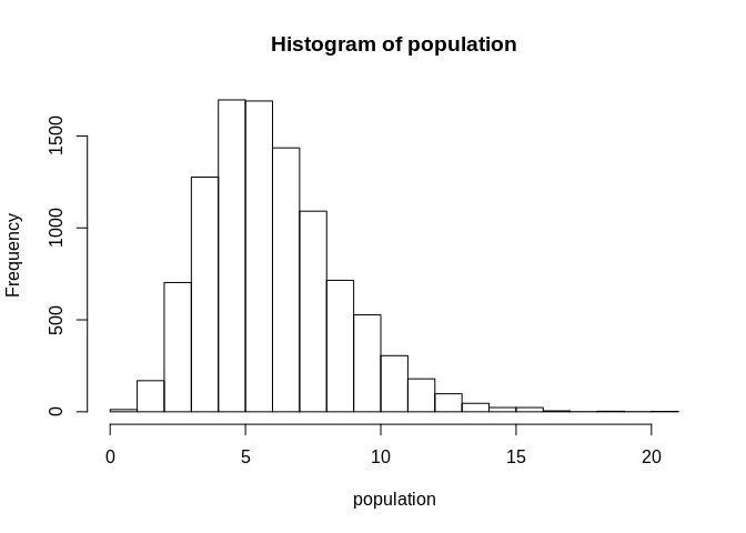

The error inflation gets even worse when dealing with skewed distribution. Thus, caution should be taken before removing outliers with these methods as to whether the distribution is not heavily skewed.

Conclusions

Outlier detection and removal should be done with care and never without a well-defined method. Data that present distributions far from a normal one should not be subjected to the methods presented here. Removing outliers with small sample sizes (eg less than 20 observations per group or condition) can inflate type I error rates substantially and should be avoided. Outlier removal must be decided without taking into account statistical significance and the same method must be applied throughout the whole study (at least to similar data). If outliers are removed, they must be rare (as a rule-of-thumb, they must account for less than 5% of the data - ideally less than 1%) and the method used to remove them as well as the number of observations removed must be clearly stated. Publishing the original data with outliers is also strongly advisable. Domain knowledge is key to determine when outliers are most likely due to error and not natural variability. Today, modern statistical techniques that are robust to extreme values exist and should be preferred whenever possible (for example, see the WRS2 package). Moreover, data that present non-normal distributions should not be forced into a normal-like distribution through outlier removal. The most important thing about outliers is to try to understand how they arise and to make efforts so that outliers don’t even appear - thus, rendering its removal unnecessary in most cases. In my experience, most outliers arise due to pre-analytical mistakes and small sample sizes. Thus, well-standardized techniques combined with parsimonious sample sizes can mitigate the issue in many cases.

References

Iglewicz, Boris, and 1944- Hoaglin David C. (David Caster). 1993. How to Detect and Handle Outliers. Book; Book/Illustrated. Milwaukee, Wis. : ASQC Quality Press.