
This is the part 2 of a series, please read part 1 before reading this.
We’ll use Recurrent Neural Networks to classify the Sentiment140 dataset into positive or negative tweets. Previously, we used a Bag of Words followed by a logistic regression classifier. This approach, however, completely ignores the semantic relationship between words as it only consider the count of each word in a tweet. Thus, we aim at considering the position of words and its complex relationships to achieve better classification.
Pre-processing
The exact same pre-processing steps will be used:
import re
import pandas as pd
import numpy as np
from matplotlib import pyplot as plt

data = pd.read_csv('training.1600000.processed.noemoticon.csv', encoding = 'ISO-8859-1', header = None)
data.columns = ['sentiment','id','date','flag','user','tweet']
def preprocess_tweets(tweet):
    tweet = re.sub(r"([A-Z]+\s?[A-Z]+[^a-z0-9\W]\b)", r"\1 <ALLCAPS> ", tweet)
    tweet = re.sub('((www\.[^\s]+)|(https?://[^\s]+))','<URL> ', tweet)
    tweet = re.sub(r"/"," / ", tweet)
    tweet = re.sub('@[^\s]+', "<USER>", tweet)
    tweet = re.sub('[^A-Za-z0-9<>/.!,?\s]+', '', tweet)
    tweet = re.sub('(([!])\\2+)', '! <REPEAT> ', tweet)
    tweet = re.sub('(([?])\\2+)', '? <REPEAT> ', tweet)
    tweet = re.sub('(([.])\\2+)', '. <REPEAT> ', tweet)
    tweet = re.sub(r'#([^\s]+)', r'<HASHTAG> \1', tweet)
    tweet = re.sub(r'(.)\1{2,}\b', r'\1 <ELONG> ', tweet)
    tweet = re.sub(r'(.)\1{2,}', r'\1)', tweet)
    tweet = re.sub(r"'ll", " will", tweet)
    tweet = re.sub(r"'s", " is", tweet)
    tweet = re.sub(r"'d", " d", tweet) # Would/Had ambiguity
    tweet = re.sub(r"'re", " are", tweet)
    tweet = re.sub(r"didn't", "did not", tweet)
    tweet = re.sub(r"couldn't", "could not", tweet)
    tweet = re.sub(r"can't", "cannot", tweet)
    tweet = re.sub(r"doesn't", "does not", tweet)
    tweet = re.sub(r"don't", "do not", tweet)
    tweet = re.sub(r"hasn't", "has not", tweet)
    tweet = re.sub(r"'ve", " have", tweet)
    tweet = re.sub(r"shouldn't", "should not", tweet)
    tweet = re.sub(r"wasn't", "was not", tweet)
    tweet = re.sub(r"weren't", "were not", tweet)
    tweet = re.sub('[\s]+', ' ', tweet)
    tweet = tweet.lower()

    return tweet
This time, however, we’ll split the data into train, test and validation sets. The validation set is used to monitor overfitting during training. The test set should be left untouched and unseen until its evaluation. It may sound counter-intuitive, but merely tweaking the model according to the validation set performance may produce indirect overfitting (indirect as the model never sees any of the validation data) and may jeopardize its generalization capability (that is, its ability to perform well in data other than what it was trained on).
from sklearn.model_selection import train_test_split

train_data, test_data = train_test_split(data, train_size = 0.8, random_state = 42)

sentiment = np.array(data['sentiment'])
tweets = np.array(data['tweet'].apply(preprocess_tweets))

sentiment_train = np.array(train_data['sentiment'])
tweets_train = np.array(train_data['tweet'].apply(preprocess_tweets))

sentiment_test = np.array(test_data['sentiment'])
tweets_test = np.array(test_data['tweet'].apply(preprocess_tweets))

train_data, val_data = train_test_split(train_data, train_size = 0.9, random_state = 42)

sentiment_train = np.array(train_data['sentiment'])
tweets_train = np.array(train_data['tweet'].apply(preprocess_tweets))

sentiment_val = np.array(val_data['sentiment'])
tweets_val = np.array(val_data['tweet'].apply(preprocess_tweets))
Just like in the previous post, we’ll count word occurrences and establish a parsimonious threshold. Words below this threshold will be replaced by the OUT tag. This way, we limit model complexity while retaining most of information (more than 95% of word occurrences). Next, we build a word2int dictionary that assigns an integer value to each word in our dictionary. PAD, OUT, EOS and SOS tokens are also included in the dictionary. However, the end-of-sentence (EOS) and start-of-sentence (SOS) ended up not being used on this model.
word2count = {}
for tweet in tweets:
    for word in re.findall(r"[\w']+|[.,!?]", tweet):
        if word not in word2count:
            word2count[word] = 1
        else:
            word2count[word] += 1

total_count = np.array(list(word2count.values()))

print(sum(total_count[total_count > 75]) / sum(total_count))

threshold = 75
words2int = {}
word_number = 0
for word, count in word2count.items():
    if count > threshold:
        words2int[word] = word_number
        word_number += 1

tokens = ['<PAD>', '<OUT>', '<EOS>', '<SOS>']

for token in tokens:
    words2int[token] = len(words2int) + 1

int2word = {w_i: w for w, w_i in words2int.items()}

print(len(words2int))
0.9551287692699321
9983
Thus, our final dictionary contains 9983 unique entries. Let’s convert all of our tweets into series of integers according to our dictionary:
tweets_train_int = []

for _tweet in tweets_train:
    ints = []
    for word in re.findall(r"[\w']+|[.,!?]", _tweet):
        if word not in words2int:
            ints.append(words2int['<OUT>'])
        else:
            ints.append(words2int[word])
    tweets_train_int.append(ints)

tweets_val_int = []

for _tweet in tweets_val:
    ints = []
    for word in re.findall(r"[\w']+|[.,!?]", _tweet):
        if word not in words2int:
            ints.append(words2int['<OUT>'])
        else:
            ints.append(words2int[word])
    tweets_val_int.append(ints)

tweets_test_int = []

for _tweet in tweets_test:
    ints = []
    for word in re.findall(r"[\w']+|[.,!?]", _tweet):
        if word not in words2int:
            ints.append(words2int['<OUT>'])
        else:
            ints.append(words2int[word])
    tweets_test_int.append(ints)


tweets_int = tweets_train_int + tweets_val_int + tweets_test_int
Our recurrent neural network receive inputs of fixed length. Therefore, our sequences will be padded (the PAD token will be added to the beginning of every tweet until it reaches our fixed length). Again, some tweets are extremely long due to repetitions and excessive punctuation. As a parsimonious length, the 99th percentile of all lengths was chosen, that is, 99% of all tweets will fit in our maximum padding length. Tweets longer than this will be truncated at the maximum length.
lens = []
for i in tweets_int:
    lens.append(len(i))

max_len = int(np.quantile(lens, 0.99))

print(max_len)
34
from keras.preprocessing.sequence import pad_sequences

pad_tweets_train = pad_sequences(tweets_train_int, maxlen = max_len, value = words2int['<PAD>'])
pad_tweets_val = pad_sequences(tweets_val_int, maxlen = max_len, value = words2int['<PAD>'])
pad_tweets_test = pad_sequences(tweets_test_int, maxlen = max_len, value = words2int['<PAD>'])

sentiment_train[sentiment_train == 4] = 1
sentiment_test[sentiment_test == 4] = 1
sentiment_val[sentiment_val == 4] = 1
Building our Neural Network
A research paper suggests that a combination of 1D convolutions with recurrent units result in a higher performance than both of these alone. Thus, we built a neural network with an architecture inspired by this research paper.
Neural networks cannot make sense of the dictionary-labeled integers for each word, so a one-hot-encoded vector is passed as its input. That is, each word becomes a 9983-dimensional vector with all values set to 0 except one: the corresponding word is the set to one. This data structure is extremely sparse and would require a staggering amount of trainable parameters. Thus, a word embedding is included as a first layer to the model.
An embedding is a form of dimensionality reduction. In the one-hot-encoded vector, every word is independent of all others, as each word has a single exclusive dimension for representation. In an embedding, each word is represented as a vector in a n-dimensional space, where n is much smaller than the number of words. This way, words are dependent on each other and, in a good embedding, semantically similar words lay closer in the embedding space. In our model, the embedding will be 200-dimensional. Learning how to embed words is not a simple task and many models use pre-trained embeddings. However, as our data consists of tweets, which contain many typos and idioms, I first wanted to use a untrained embedding, which is trained simultaneously with the model.
After the embedding layer, two parallel networks exist: one is a series of three 1D convolutions that can master relationships between adjacent words (remember that the words will be represented as a vector containing its meaning laying in a 200-dimensional space); the other path is a two-layered recurrent neural network composed of GRU units. GRUs are fairly recent, they are easier to train than the classic LSTM units (as they have fewer parameters) and often result in similar performance. Thus, I wanted to give the still young GRU a try.
A quite large dropout (0.5 rate) is used after the GRU layers as recurrent neural networks easily overfit. This rate is still smaller than the one suggested on the paper (0.7), although they used LSTM units.
The model architecture is represented on the scheme below:
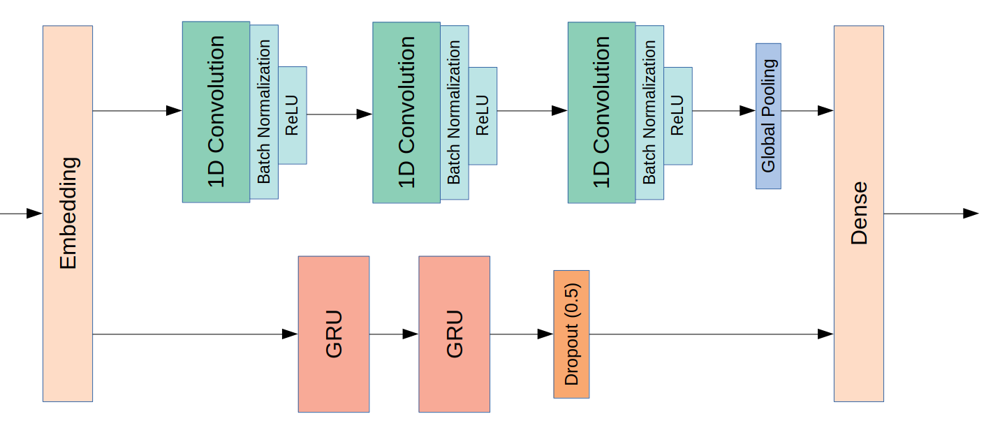
Keras functional API must be used due to parallel layers. The result of both 1D convolutions and GRUs is concatenated and followed by a 1-unit output dense layer. The Adam optimizer with soft weight decay will be used.
import keras
from keras.layers import Dense, Dropout, Conv1D, GRU, Embedding, Activation,\
BatchNormalization, concatenate, Input, GlobalAveragePooling1D
from keras.optimizers import Adam
from keras.models import Model

inputs = Input(shape = (34,), dtype = 'int32')

emb = Embedding(9983, 200, input_length = 34)(inputs)
emb_drop = Dropout(0)(emb)

out1 = Conv1D(128, 3)(emb_drop)
out1 = BatchNormalization()(out1)
out1 = Activation('relu')(out1)
out1 = Conv1D(64, 4)(out1)
out1 = BatchNormalization()(out1)
out1 = Activation('relu')(out1)
out1 = Conv1D(64, 3)(out1)
out1 = BatchNormalization()(out1)
out1 = Activation('relu')(out1)
out1 = GlobalAveragePooling1D()(out1)
out1_drop = Dropout(0)(out1)

out2 = GRU(128, return_sequences = True)(emb_drop)
out2 = GRU(128)(out2)
out2_drop = Dropout(0.5)(out2)

out_main = concatenate([out1_drop, out2_drop])
out_main = Dense(1, activation = 'sigmoid')(out_main)

model = Model(inputs = inputs, outputs = out_main)

early = keras.callbacks.EarlyStopping(monitor='val_loss', min_delta=1e-3, patience=1, verbose=0, mode='auto', baseline=None, restore_best_weights=True)
board = keras.callbacks.TensorBoard(log_dir='./logs_paper', histogram_freq=0, batch_size=64, write_graph=True, write_grads=False, write_images=False, update_freq= 1280)
check = keras.callbacks.ModelCheckpoint('model_paper.weights.{epoch:02d}-{val_loss:.4f}.hdf5', monitor='val_loss', verbose=0, save_best_only=False, save_weights_only=False, mode='auto', period=1)

model.compile(optimizer = Adam(lr = 1e-3, decay = 5e-6), loss = 'binary_crossentropy', metrics = ['accuracy'])

print(model.summary())
__________________________________________________________________________________________________
Layer (type)                    Output Shape         Param #     Connected to
==================================================================================================
input_7 (InputLayer)            (None, 34)           0
__________________________________________________________________________________________________
embedding_7 (Embedding)         (None, 34, 200)      1996600     input_7[0][0]
__________________________________________________________________________________________________
dropout_19 (Dropout)            (None, 34, 200)      0           embedding_7[0][0]
__________________________________________________________________________________________________
conv1d_19 (Conv1D)              (None, 32, 128)      76928       dropout_19[0][0]
__________________________________________________________________________________________________
batch_normalization_19 (BatchNo (None, 32, 128)      512         conv1d_19[0][0]
__________________________________________________________________________________________________
activation_19 (Activation)      (None, 32, 128)      0           batch_normalization_19[0][0]
__________________________________________________________________________________________________
conv1d_20 (Conv1D)              (None, 29, 64)       32832       activation_19[0][0]
__________________________________________________________________________________________________
batch_normalization_20 (BatchNo (None, 29, 64)       256         conv1d_20[0][0]
__________________________________________________________________________________________________
activation_20 (Activation)      (None, 29, 64)       0           batch_normalization_20[0][0]
__________________________________________________________________________________________________
conv1d_21 (Conv1D)              (None, 27, 64)       12352       activation_20[0][0]
__________________________________________________________________________________________________
batch_normalization_21 (BatchNo (None, 27, 64)       256         conv1d_21[0][0]
__________________________________________________________________________________________________
activation_21 (Activation)      (None, 27, 64)       0           batch_normalization_21[0][0]
__________________________________________________________________________________________________
gru_17 (GRU)                    (None, 34, 128)      126336      dropout_19[0][0]
__________________________________________________________________________________________________
global_average_pooling1d_7 (Glo (None, 64)           0           activation_21[0][0]
__________________________________________________________________________________________________
gru_18 (GRU)                    (None, 128)          98688       gru_17[0][0]
__________________________________________________________________________________________________
dropout_20 (Dropout)            (None, 64)           0           global_average_pooling1d_7[0][0]
__________________________________________________________________________________________________
dropout_21 (Dropout)            (None, 128)          0           gru_18[0][0]
__________________________________________________________________________________________________
concatenate_7 (Concatenate)     (None, 192)          0           dropout_20[0][0]
                                                                 dropout_21[0][0]
__________________________________________________________________________________________________
dense_7 (Dense)                 (None, 1)            193         concatenate_7[0][0]
==================================================================================================
Total params: 2,344,953
Trainable params: 2,344,441
Non-trainable params: 512
__________________________________________________________________________________________________
The model contains 2.3 million trainable parameters and takes a fairly large time to train using a mid-performance CUDA-capable GPU. Extra dropout layers with the rate set to 0 (rendering their presence irrelevant) were added to possibly tweak dropout rates during training.
model.fit(x = pad_tweets_train, y = sentiment_train,\
          validation_data = (pad_tweets_val, sentiment_val),\
          batch_size = 64, epochs = 20,\
          callbacks = [early, board, check])
Epoch 1/20
1152000/1152000 [==============================] - 2382s 2ms/step - loss: 0.3939 - acc: 0.8220 - val_loss: 0.3654 - val_acc: 0.8380
Epoch 2/20
1152000/1152000 [==============================] - 2426s 2ms/step - loss: 0.3480 - acc: 0.8473 - val_loss: 0.3538 - val_acc: 0.8432
Epoch 3/20
1152000/1152000 [==============================] - 2596s 2ms/step - loss: 0.3225 - acc: 0.8608 - val_loss: 0.3527 - val_acc: 0.8441
Epoch 4/20
1152000/1152000 [==============================] - 2747s 2ms/step - loss: 0.2984 - acc: 0.8734 - val_loss: 0.3643 - val_acc: 0.8411
After the third epoch, the model reached its best performance on the validation set. The EarlyStopping callback makes sure that this is the model that is kept under the model variable.
Model Evaluation
from copy import deepcopy as dc
from sklearn.metrics import roc_auc_score, f1_score

pred = model.predict(pad_tweets_test)
pred_label = dc(pred)
pred_label[pred_label > 0.5] = 1
pred_label[pred_label <= 0.5] = 0

auc = roc_auc_score(sentiment_test, pred)
f1 = f1_score(sentiment_test, pred_label)
print('AUC: {}'.format(np.round(auc, 4)))
print('F1-score: {}'.format(np.round(f1, 4)))
AUC: 0.9231
F1-score: 0.8452
The best AUC achieved with the bag of words approach was 0.8782, showing that the positional information added in this model really boosts performance. Still, it was a very mild improvement. This is expected as improvements in performance get exponentially more expensive with better models.
As in the first part of this post series, the top false positives and false negatives are actually mislabeled data. Thus, we’ll take a peek at random false positive or negative examples, without actually choosing the most “incorrect” ones.
- True Positives
from random import sample

pos_indices = sentiment_test == 1
pos_predicted = (pred > 0.5).reshape((-1))
true_positives = pos_indices & pos_predicted

samples = sample(range(sum(true_positives)), 5)
print(tweets_test[true_positives][samples])
print(pred.reshape((-1))[true_positives][samples])
| Tweet | Positive Probability |
|---|---|
| ‘feeling better about everything thank you booze!’ | 0.9616 |
| ‘some writing, some dusting, and then work 59 with tricia! ‘ | 0.6634 |
| ‘ |
0.9469 |
| ‘ |
0.8898 |
| ‘ |
0.8991 |
- True Negatives
neg_indices = sentiment_test == 0
neg_predicted = (pred <= 0.5).reshape((-1))
true_negatives = neg_indices & neg_predicted

samples = sample(range(sum(true_positives)), 5)
print(tweets_test[true_negatives][samples])
print(pred.reshape((-1))[true_negatives][samples])
| Tweet | Positive Probability |
|---|---|
| ‘well ive now got a chest infection, and it hurts like a bitch i want <allcaps> kfc <allcaps> ‘ | 0.0102 |
| ‘a bee stung me in the finger! its so swollen that i dont have a fingerprint. ‘ | 0.0077 |
| ‘i miss having tcm <allcaps> ‘ | 0.0141 |
| ‘kittens are going soon. sad times. i love them too much ‘ | 0.4847 |
| ’<user> i took 2 weeks off work for in the sun, instead im lieing here trying to use this bastard twitter, gr <elong> i should be raving ‘ | 0.2338 |
- False Positives
neg_indices = sentiment_test == 0
pos_predicted = (pred > 0.5).reshape((-1))
false_positives = neg_indices & pos_predicted

samples = sample(range(sum(false_positives)), 10)
print(tweets_test[false_positives][samples])
print(pred.reshape((-1))[false_positives][samples])
| Tweet | Positive Probability |
|---|---|
| ’<user> with 1 / 40th of that following alone, i could stay on twitter 24 / 7 the only stress to tire me would come from coulterites! ‘ | 0.7520 |
| ’<user> not even in the land of ketchup, thats just wrong. did u ever try the ketchup fries?’ | 0.6687 |
| ’<user> thanks girlie i need it. <repeat> theres a lot to do ‘ | 0.7414 |
| ’<user> hi ryan! why you are getting so unfashionable lately? ‘ | 0.8097 |
| ‘i dont know what i am doing on here. wow i joined the new fad ‘ | 0.8859 |
| ’<user> thats okay. <repeat> it will take a couple hours of intense therapy to get over it, but ill manage somehow ‘ | 0.9083 |
| ’? <repeat> quotbest video <url> ? <repeat> ? <repeat> ? <repeat> ? <repeat> , ? <repeat> ? <repeat> ? <repeat> ? <repeat> ? <repeat> ! i already clicked it <url> ‘ | 0.5936 |
| ‘wii fit day 47. hang over prevented wii this morning. late night work meant i wasnt home til near midnight. 15 min walk then situps. ‘ | 0.6522 |
| ’<user> were gettin alot of rain. we must be getting yours! ‘ | 0.6998 |
| ‘im tired didnt do anything all day! except went to the craft store to get some hemp string ‘ | 0.8360 |
- False Negatives
pos_indices = sentiment_test == 1
neg_predicted = (pred <= 0.5).reshape((-1))
false_negatives = pos_indices & neg_predicted

samples = sample(range(sum(false_negatives)), 10)
print(tweets_test[false_negatives][samples])
print(pred.reshape((-1))[false_negatives][samples])
| Tweet | Positive Probability |
|---|---|
| ‘okay, a bath is a must. and then studying! i really have no life.’ | 0.2401 |
| ’<user> so you hate me ‘ | 0.3220 |
| ‘catching up on my reading. <repeat> twitter n bf break ‘ | 0.4715 |
| ’<user> good thing when quotdj heroquot video game comes out there will be no more wanna be djs ‘ | 0.4940 |
| ‘gained 1 follower. i need more. haha! ‘ | 0.4358 |
| ‘thanks <user> it is the avatar i started with. hope all is well. had more storms here today though nothi. <repeat> )<url> ‘ | 0.2736 |
| ‘so <elong> have to piss right now, cant find the energy to want to unleash the fury ‘ | 0.0265 |
| ‘oh snap. <repeat> kinda nuts right now. <repeat> <user> ive told at least 27 thanks babes.’ | 0.4799 |
| ‘ahh, worried about tomorrow. <repeat> will they turn up. <repeat> ? haha ‘ | 0.3653 |
| ‘my eyes are red. should sleep but dnt feel like it, haha. lilee is sitting on my chair so i have to sit on my bed ‘ | 0.1993 |
We can see that true positives and negatives are indeed positive and negative, respectively. It is worth mentioning one example from true positives (“some writing, some dusting, and then work 59 with tricia!”) which is not obviously positive and, accordingly, received a lower probability. From the negatives, the tweet “kittens are going soon. sad times. i love them too much” remained almost uncertain to the model probably due to the “i love them too much” part.
Some false positives or negatives don’t have an explicit feeling to them - e.g “<user> were gettin alot of rain. we must be getting yours!”, “catching up on my reading. <repeat> twitter n bf break”; without the label, its hard to classify them (most likely because emoji information was lost, and so the model incorrectly classified them but with probabilities close to 0.5. Some other mistakes are actually mislabeled data (e.g. “okay, a bath is a must. and then studying! i really have no life.”, “
There are, of course, some obvious mistakes, such as “wii fit day 47. hang over prevented wii this morning. late night work meant i wasnt home til near midnight. 15 min walk then situps” (incorrectly classified as a positive).
It’s worth mentioning that the complex nature of our model gives it a black box nature. That is, it’s very hard to know why a tweet was classified in some particular way. For example, the tweets “<user> not even in the land of ketchup, thats just wrong. did u ever try the ketchup fries?” (probability: 0.6687) and “<user> hi ryan! why you are getting so unfashionable lately?” (probability: 0.8097) were false positives, yet they can be classified as positives if we consider they’re funny. Still, it’s very far-fetched to assume that the model learned a sense of humor. It’s also a mistery why the tweet “<user> thats okay.
Finally, it’s perceivable that this model has a greater ability to detect sentiment without obvious words (such as love, hate, pain, happy). This is the major improvement from the bag of words approach.
Leave a comment