
Sentiment classification is somewhat of a trend in NLP; it consists of classifying small texts according to its sentiment connotation: a positive or negative feeling. Today we’ll use the Sentiment140 dataset to train a classifier model in python. The dataset consists of 1.6 million sentiment-labeled tweets. The encoding must be manually set.
import re
import pandas as pd
import numpy as np
from matplotlib import pyplot as plt

data = pd.read_csv('training.1600000.processed.noemoticon.csv', encoding = 'ISO-8859-1', header = None)
data.columns = ['sentiment','id','date','flag','user','tweet']
Let’s take a look at some tweet examples by sentiment:
from random import sample

data_positive = data.loc[data['sentiment'] == 4]

pd.options.display.max_colwidth = 200

data_positive.iloc[sample(range(len(data_positive)), 10)]['tweet']
882683                                                                      Flickr is uploading... Oooh, and these pics count towards my 101 things!
1427010                                                                                                         @mrdirector09 That's why you have me
803819                                                                                            @michaelgrainger lmao! I understand bro...trust me
1326235    @kyleandjackieo I.e. I don't need to know when you're getting a coffee, and I don't need to know all your deep thoughts about everything.
1490141                                                                                                                                At sushi land
1348059                                                                              just realized my birthday isnt that far away a month and 3 days
1439467                                                                                      @uhhitsangelaa thats good. glad ur feeling better girl!
1022555                                                                                                                      @mikecane Thanks, Mike!
973136                                                                                    i just found out that my name means god's grace in hebrew.
806094                                             @rahnocerous tired. yr 12 is killing me, albeit slowly. 2 days left and im on 2 week break though
Name: tweet, dtype: object
from random import sample

data_negative = data.loc[data['sentiment'] == 0]

pd.options.display.max_colwidth = 200

data_negative.iloc[sample(range(len(data_positive)), 10)]['tweet']
609074                                                                                  The weather is blowing mines right now and I'm in traffic
195300                                                                      @keza34 oh i havent, ive bn sat at home with withdrawels, so not good
103236                                          Only powder pink slipon vans would have completed this look. I rushed out and forgot my hair ties
760227              @jenleighbarry Hey Jen! Sadly  no.. guessing you are!? Awsomeness! Can hear the click-click of your focused eye going to work!
163747    Home. Don't think i'll wake up at 5. :-p I had set an alarm for 6 in the kids' room & forgot to turn it off. I feel bad about that.
112837                                                                          i woke up earlier than i wanted to thanks to Prince  parade todayy
430999                                 @janiceromero same thing happened to me..  it either you not use Akismet or just check your comments daily.
268119                                                                  ok...am i java rookie...i knw...bt i hope ds openCMS docs make some sense
61601                                                                            @clara018 yeah! my day seemed to pass so fast without him update
147459                                  @cloverdash He's playing Juan Ignacio Chela...who's good on clay.  very annoying. Fingers crossed though!
Name: tweet, dtype: object
We can see that not all tweets are obviously positive or negative, the less obvious ones will be a challenge to our classifier.
Pre-Processing
Pre-processing is a huge step in our analysis, as it directly influences the model’s performance. We’ll use python regex to indicate words that are all caps, replace URLs for URL, user mentions with USER, remove all special symbols, indicate punctuation repetitions with REPEAT, hashtags with HASHTAG and word end elongations (e.g. heeyyyyyyy) with ELONG. English contractions are split, extra spaces removed and, finally, everything is set to lower case.
def preprocess_tweets(tweet):
    #Detect ALLCAPS words
    tweet = re.sub(r"([A-Z]+\s?[A-Z]+[^a-z0-9\W]\b)", r"\1 <ALLCAPS> ", tweet)
    #Remove URLs
    tweet = re.sub('((www\.[^\s]+)|(https?://[^\s]+))','<URL> ', tweet)
    #Separate words that are joined by / (e.g. black/brown)
    tweet = re.sub(r"/"," / ", tweet)
    #Remove user mentions
    tweet = re.sub('@[^\s]+', "<USER>", tweet)
    #Remove all special symbols
    tweet = re.sub('[^A-Za-z0-9<>/.!,?\s]+', '', tweet)
    #Detect puncutation repetition
    tweet = re.sub('(([!])\\2+)', '! <REPEAT> ', tweet)
    tweet = re.sub('(([?])\\2+)', '? <REPEAT> ', tweet)
    tweet = re.sub('(([.])\\2+)', '. <REPEAT> ', tweet)
    #Remove hashtags
    tweet = re.sub(r'#([^\s]+)', r'<HASHTAG> \1', tweet)
    #Detect word elongation (e.g. heyyyyyy)
    tweet = re.sub(r'(.)\1{2,}\b', r'\1 <ELONG> ', tweet)
    tweet = re.sub(r'(.)\1{2,}', r'\1)', tweet)
    #Expand english contractions
    tweet = re.sub(r"'ll", " will", tweet)
    tweet = re.sub(r"'s", " is", tweet)
    tweet = re.sub(r"'d", " d", tweet) # Would/Had ambiguity
    tweet = re.sub(r"'re", " are", tweet)
    tweet = re.sub(r"didn't", "did not", tweet)
    tweet = re.sub(r"couldn't", "could not", tweet)
    tweet = re.sub(r"can't", "cannot", tweet)
    tweet = re.sub(r"doesn't", "does not", tweet)
    tweet = re.sub(r"don't", "do not", tweet)
    tweet = re.sub(r"hasn't", "has not", tweet)
    tweet = re.sub(r"'ve", " have", tweet)
    tweet = re.sub(r"shouldn't", "should not", tweet)
    tweet = re.sub(r"wasn't", "was not", tweet)
    tweet = re.sub(r"weren't", "were not", tweet)
    #Remove extra spaces
    tweet = re.sub('[\s]+', ' ', tweet)
    #Lower case
    tweet = tweet.lower()

    return tweet
Let’s use train_test_split to split our data into training and testing data while applying our preprocess function.
from sklearn.model_selection import train_test_split

train_data, test_data = train_test_split(data, train_size = 0.8, random_state = 42)

sentiment = np.array(data['sentiment'])
tweets = np.array(data['tweet'].apply(preprocess_tweets))

sentiment_train = np.array(train_data['sentiment'])
tweets_train = np.array(train_data['tweet'].apply(preprocess_tweets))

sentiment_test = np.array(test_data['sentiment'])
tweets_test = np.array(test_data['tweet'].apply(preprocess_tweets))
We’ll build a word2count dictionary that will have a key entry for each word found in the data and a value corresponding to how many times that word was seen. Later, a parsimonious threshold that included slightly more than 95% of word occurrences was chosen.
word2count = {}
for tweet in tweets:
    for word in re.findall(r"[\w']+|[.,!?]", tweet):
        if word not in word2count:
            word2count[word] = 1
        else:
            word2count[word] += 1

total_count = np.array(list(word2count.values()))

print(sum(total_count[total_count > 75]) / sum(total_count))
0.9551287692699321
Zipf’s Law is an empirical approximation which states that the second most frequent word in a language is used half as frequently as the first one, the third one, a third of the frequency of the first one and so on. Mathematically, Zipf’s Law can be defined as  , where Pn represents the frequency of the n-th most frequent word and alpha is approximately 1. This relationship can be seen as a line in a log-log plot with the y-axis as log(count) and x-axis as log(rank) of words:
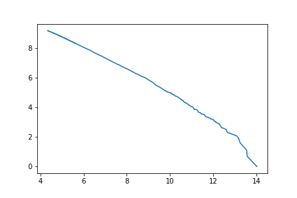
Thus, word frequency exponentially decreases and words that are rarely seen provide little to none information to our model and make it much more complex and sparse. Therefore, only relatively frequent words are included while still holding most of information.
Vectorizing
We’ll build a bag of words, in which each tweet will become a vector of length n, where n is the number of words in our dictionary, and the values of this vector correspond to how many times that word is seen in that tweet. This approach, however, has a huge disadvantage: very frequent words (such as the and a) will almost always have the highest counts, while actually holding little information. The TF-IDF (term frequency times inverse document frequency) approach tackles this issue by using a different count value: we’ll use a simple approach and multiply the text (tweet) frequency of a word by log [ n / df(d, t) ] + 1, where n is the number of documents and df(d, t) is the number of documents which contain the word. Thus, the transformed count value will indicate which words stand out as most unique and defining on each tweet.
from sklearn.feature_extraction.text import TfidfVectorizer

vectorizer = TfidfVectorizer(min_df = 75)
vectorizer.fit(tweets)

tweets_bow_train = vectorizer.transform(tweets_train)
tweets_bow_test = vectorizer.transform(tweets_test)
Next, a logistic regression will be the model of choice to classify the data. As the model will receive a huge input vector while having to output a single value, it’s reasonable that the weights should be relatively sparse, that is, many words should have little to no influence on the output. Thus, we’ll use L1 penalty to ensure sparsity in the model. The C parameter is the inverse of regularization strength, that is, lower C values result in a stronger regularization and sparser solutions. We’ll try three different C values. A fourth model with L2 penalty and C = 1 (default value) will be fit for comparison.
from sklearn.linear_model import LogisticRegression

regressor1 = LogisticRegression(C = 1, penalty = 'l1', solver = 'liblinear',\
                                multi_class = 'ovr', random_state = 42)
regressor1.fit(tweets_bow_train_idf, sentiment_train)

regressor2 = LogisticRegression(C = 0.5, penalty = 'l1', solver = 'liblinear',\
                                multi_class = 'ovr', random_state = 42)
regressor2.fit(tweets_bow_train_idf, sentiment_train)

regressor3 = LogisticRegression(C = 0.1, penalty = 'l1', solver = 'liblinear',\
                                multi_class = 'ovr', random_state = 42)
regressor3.fit(tweets_bow_train_idf, sentiment_train)

regressor4 = LogisticRegression(solver = 'liblinear', multi_class = 'ovr',\
                                random_state = 42)
regressor4.fit(tweets_bow_train_idf, sentiment_train)
We’ll use area under the curve (AUC) and F1-score to measure models’ performance.
from sklearn.metrics import roc_auc_score, f1_score

pred1 = regressor1.predict(tweets_bow_test)
pos_prob1 = regressor1.predict_proba(tweets_bow_test)[:, 1]
auc1 = roc_auc_score(sentiment_test, pos_prob1)
f11 = f1_score(sentiment_test, pred1, pos_label=4)

pred2 = regressor2.predict(tweets_bow_test)
pos_prob2 = regressor2.predict_proba(tweets_bow_test)[:, 1]
auc2 = roc_auc_score(sentiment_test, pos_prob2)
f12 = f1_score(sentiment_test, pred2, pos_label=4)

pred3 = regressor3.predict(tweets_bow_test)
pos_prob3 = regressor3.predict_proba(tweets_bow_test)[:, 1]
auc3 = roc_auc_score(sentiment_test, pos_prob3)
f13 = f1_score(sentiment_test, pred3, pos_label=4)

pred4 = regressor4.predict(tweets_bow_test)
pos_prob4 = regressor4.predict_proba(tweets_bow_test)[:, 1]
auc4 = roc_auc_score(sentiment_test, pos_prob4)
f14 = f1_score(sentiment_test, pred4, pos_label=4)
Model 1:
AUC: 0.8782442518806748
F1: 0.8017438980490371
Model 2:
AUC: 0.878181401427863
F1: 0.8021068750172958
Model 3:
AUC: 0.8724711782629141
F1: 0.7978355389550899
Model 4:
AUC: 0.878032003703207
F1: 0.8012445320682644
Model 1 is the best one AUC-wise, while model 2 is the best one according to F1 score. Let’s see the sparsity on each model:
sparsity1 = np.mean(regressor1.coef_.ravel() == 0) * 100
sparsity2 = np.mean(regressor2.coef_.ravel() == 0) * 100
sparsity3 = np.mean(regressor3.coef_.ravel() == 0) * 100
sparsity4 = np.mean(regressor4.coef_.ravel() == 0) * 100

print('Sparsity with L1 and C = 1: %.2f%%' % sparsity1)
print('Sparsity with L1 and C = 0.5: %.2f%%' % sparsity2)
print('Sparsity with L1 and C = 0.1: %.2f%%' % sparsity3)
print('Sparsity with L2 and C = 1: %.2f%%' % sparsity4)
Sparsity with L1 and C = 1: 15.51%
Sparsity with L1 and C = 0.5: 29.29%
Sparsity with L1 and C = 0.1: 72.18%
Sparsity with L2 and C = 1: 0.00%
It’s quite amazing that even with 72.18% of coefficients set to 0, model 3 was still able to achieve a performance almost identical to much more complex models. Also, as guessed, sparsity rises model performance and makes it simpler, as the L2 model with no sparsity is much more complex and performs a bit worse according to both metrics.
Interpreting the model
Let’s see which words have the largest contribution for both positive and negative sentiment. The third model will be used as it’s more sparse and allows for better interpretation.
coefs = np.array(regressor3.coef_.ravel())

sorting = coefs.argsort()

high_coefs = []
high_words = []
for i in range(-1, -21, -1):
    high_coefs.append(coefs[sorting[i]])
    temp = np.zeros(coefs.shape[0])
    temp[sorting[i]] = 1
    high_words.append(vectorizer.inverse_transform(temp)[0][0])

low_coefs = []
low_words = []
for i in range(20):
    low_coefs.append(coefs[sorting[i]])
    temp = np.zeros(coefs.shape[0])
    temp[sorting[i]] = 1
    low_words.append(vectorizer.inverse_transform(temp)[0][0])

    high_coefs = [high_coefs]
    low_coefs = [low_coefs]

    high_coefs = np.round(high_coefs, 1)
    low_coefs = np.round(low_coefs, 1)

    fig, ax = plt.subplots(figsize = (10, 2))
    im = ax.imshow(high_coefs, cmap = 'YlGn')
    ax.set_xticks(np.arange(len(high_words)))
    ax.set_xticklabels(list(high_words))

    plt.setp(ax.get_xticklabels(), rotation=45, ha="right",
             rotation_mode="anchor")
    ax.axes.get_yaxis().set_visible(False)
    for i in range(20):
        text = ax.text(i, 0, high_coefs[0][i],
                       ha="center", va="center", color="black")
    fig.tight_layout()
    plt.savefig('highest_heatmap.png', dpi = 150)

    fig, ax = plt.subplots(figsize = (10, 2))
    im = ax.imshow(low_coefs, cmap = 'PuBu_r')
    ax.set_xticks(np.arange(len(low_words)))
    ax.set_xticklabels(list(low_words))

    plt.setp(ax.get_xticklabels(), rotation=45, ha="right",
             rotation_mode="anchor")
    ax.axes.get_yaxis().set_visible(False)

    for i in range(20):
        text = ax.text(i, 0, low_coefs[0][i],
                       ha="center", va="center", color="black")
    fig.tight_layout()
    plt.savefig('lowest_heatmap.png', dpi = 150)
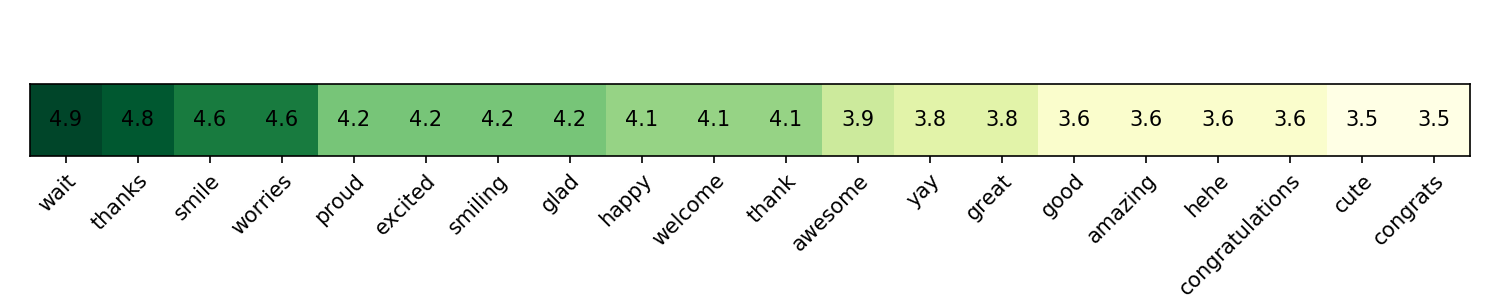
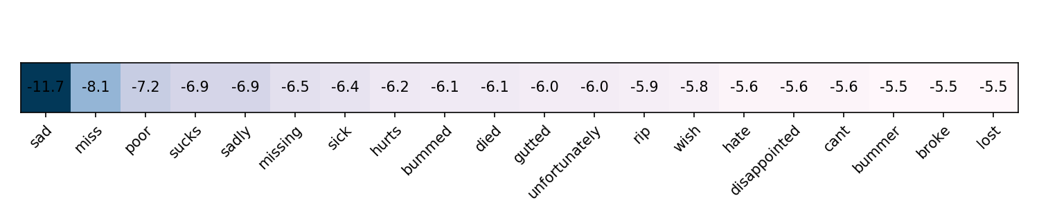
Many words are quite predictable. However, worries stands out among positive ones. Still, we can think that tweets containing worries talk about it lightly, while the word worried might have a negative connotation instead.
Let’s take a look at the 10 most correct positives:
pos_indices = sentiment_test == 4
pos_predicted = pos_prob1 > 0.5
true_positives = pos_indices & pos_predicted
true_positives_rank = np.argsort(pos_prob1[true_positives])
print(tweets_test[true_positives][true_positives_rank[range(-1, -11, -1)]])
['<user> <url> <elong> you look great. and happy. smiling is good. haha. i love your smile.'
'<user> glad it makes you happy. smile '
'<user> welcome and thank you for the followfriday! '
'<user> <user> happy birthday. we love you! thank you '
'<user> yay! <repeat> thanks for the followfriday love! <repeat> '
'<user> welcome home! im glad you had a great time, thanks for the amazing updates '
'<user> im glad you enjoy! thanks!'
'<user> yay <elong> ! thank you! youre awesome! <repeat> '
'<user> your welcome! thanks for sharing the great quote. '
'waves good morning and smiles her best smile! <url> ']
Top 10 true negatives:
neg_indices = sentiment_test == 0
neg_predicted = pos_prob1 <= 0.5
true_negatives = neg_indices & neg_predicted
true_negatives_rank = np.argsort(pos_prob1[true_negatives])
print(tweets_test[true_negatives][true_negatives_rank[range(10)]])
['is sad. i miss u . <repeat> '
'i cant believe farrah fawcett died! so sad '
'rip <allcaps> farrah fawcett! this is so sad '
'so sad to hear farrah fawcett died '
'<user> i had boatloads of sharpies and i didnt go! <repeat> sad sad sad sad so very sad. '
' sad awkwardness' 'im sad. <repeat> i miss my <user> '
'sad i dont know why i sad ' 'sad sorrow weary disappointed '
'i hate i missed roo im so sad ']
Top 10 false negatives:
pos_indices = sentiment_test == 4
neg_predicted = pos_prob1 <= 0.5
false_negatives = pos_indices & neg_predicted
false_negatives_rank = np.argsort(pos_prob1[false_negatives])
print(tweets_test[false_negatives][false_negatives_rank[range(10)]])
['<user> <allcaps> dont be sad. it doesnt make me sad '
'im not sad anymore ' '<user> that is sad! '
'dubsteppin. miss my lovies. '
'saw quotdrag me to hellquot sadly it scared me <elong> hate the ending. '
'btw, bye <user> dang! wish u went along wit them. <repeat> sad sad.'
'the saddest person is texting me telling me about how sad my life is and is getting nothing right, now shes sad '
'<user> poor girl, the fever is horrible! i hate it! get well soon bama! '
'<user> your sad ' '<user> coucou miss ']
Top 10 false positives:
neg_indices = sentiment_test == 0
pos_predicted = pos_prob1 > 0.5
false_positives = neg_indices & pos_predicted
false_positives_rank = np.argsort(pos_prob1[false_positives])
print(tweets_test[false_positives][false_positives_rank[range(-1, -11, -1)]])
['<user> cool! thank you thank you '
'<user> hey say me something haha now that you in love, love, love 8 forget about me? haha luv ya and im so happy because u happy'
'<user> i love you,i love you,i love you youre the most beautiful and sweet girl ever.'
'thank you lol' 'wait for a wonderful day ' '<user> thank you'
'<user> thank you ' '<user> thank you lovie. ' '<user> thank you. '
'<user> thanks. ']
Here we can see that most of these false positives/negatives probably are actually real negatives/positives. This suggests that there’s mislabeled data in the dataset. Moreover, this shows that the model has a good capacity of generalization, as it correctly classified mislabeled data.
This whole project shows that even a simple model, such as logistic regression, may have a very satisfactory performance with great generalization. Thus, it’s always best practice to begin with a simple model. On the following posts, I’ll use recurrent neural networks to tackle this task.
Leave a comment