Exploring Fractals With Pytorch

FracLac is a great package for fractal analysis in ImageJ. Unfortunately, no similar Python package is available. There are pieces of code that perform the box-counting algorithm.

Most implementations use the numpy reduceat function. However, this does not scale well, especially in 3 dimensions. Thus, here we use PyTorch to make use of GPU performance on 3D fractal analysis.

Generating Fractals

I used the quintic formula to generate a three-dimensional Mandelbulb pseudofractal. The params variable can be freely changed to generate different Mandelbulbs. Numba just-in-time compiler is used to make the code more efficient. Still, it is quite inefficient.

import numpy as np
from copy import deepcopy as dc
from numba import jit

@jit
def mandelbrot(x, y, z, x0, y0, z0, maxiter, params):
    A, B, C, D = params
    for n in range(maxiter + 1):
        if abs(x - x0) + abs(y - y0) + abs(z - z0) > 2:
            return n
        x = x**5 - 10*(x**3)*(y**2 + A*y*z + z**2) + 5*x*(y**4 + B*(y**3)*z + C*(y**2)*(z**2) + B*y*(z**3) + z**4) + D*(x**2)*y*z*(y+z) + x0
        y = y**5 - 10*(y**3)*(x**2 + A*x*z + z**2) + 5*y*(z**4 + B*(z**3)*x + C*(z**2)*(x**2) + B*z*(x**3) + x**4) + D*(y**2)*z*x*(z+x) + y0
        z = z**3 - 10*(z**3)*(x**2 + A*x*y + y**2) + 5*z*(x**4 + B*(x**3)*y + C*(x**2)*(y**2) + B*x*(y**3) + y**4) + D*(z**2)*x*y*(x+y) + z0
    return 0

# Draw our image
@jit
def mandelbrot_set(xmin, xmax, ymin, ymax, zmin, zmax, w, h, d, maxiter, params):
    r1 = np.linspace(xmin, xmax, w)
    r2 = np.linspace(ymin, ymax, h)
    r3 = np.linspace(zmin, zmax, d)
    n3 = np.empty((w, h, d))
    for i in range(w):
        for j in range(h):
            for k in range(d):
                x, y, z = r1[i], r2[j], r3[k]
                x0, y0, z0 = dc(x), dc(y), dc(z)
                n3[i,j, k] = mandelbrot(x, y, z, x0, y0, z0, maxiter, params)
    return (r1, r2, r3, n3)


def mandelbrot_image(dims, params, width = 20, height = 20, depth = 20, maxiter=64):
    xmin, xmax, ymin, ymax, zmin, zmax = dims
    dpi = 50
    img_width = dpi * width
    img_height = dpi * height
    img_depth = dpi * depth
    _, _, _, frac = mandelbrot_set(xmin, xmax, ymin, ymax, zmin, zmax, img_width, img_height, img_depth, maxiter, params)
    return frac

if __name__ == '__main__':
    dims = (-2, 2, -2, 2, -2, 2)
    params = (1, 0, 1, 0)
    frac = mandelbrot_image(dims, params, 10, 10, 10, 30)

Here we present an example with (1, 0, 1, 0) parameters. The code to generate an animated GIF with pyplot.imshow is presented below:

import matplotlib.pyplot as plt
import matplotlib.animation as animation
from copy import deepcopy as dc

frac_img = dc(frac)
frac_img[frac_img < 2] = 0

fig = plt.figure()

# ims is a list of lists, each row is a list of artists to draw in the
# current frame; here we are just animating one artist, the image, in
# each frame
ims = []
for i in range(int(frac_img.shape[-1]/5)):
    im = plt.imshow(frac_img[:, :, i*5]**(1/2), animated=True, cmap = 'bone')
    ims.append([im])

ani = animation.ArtistAnimation(fig, ims, interval=75, blit=True,
                                repeat_delay=0)

ani.save('./frac_animation.gif', writer='imagemagick', fps = 30)

The square-root is used to reduce the image contrast and enhance visualization. The image represents a sliding slice of the image on the z-axis, just like a tomography.

Fractal Analysis

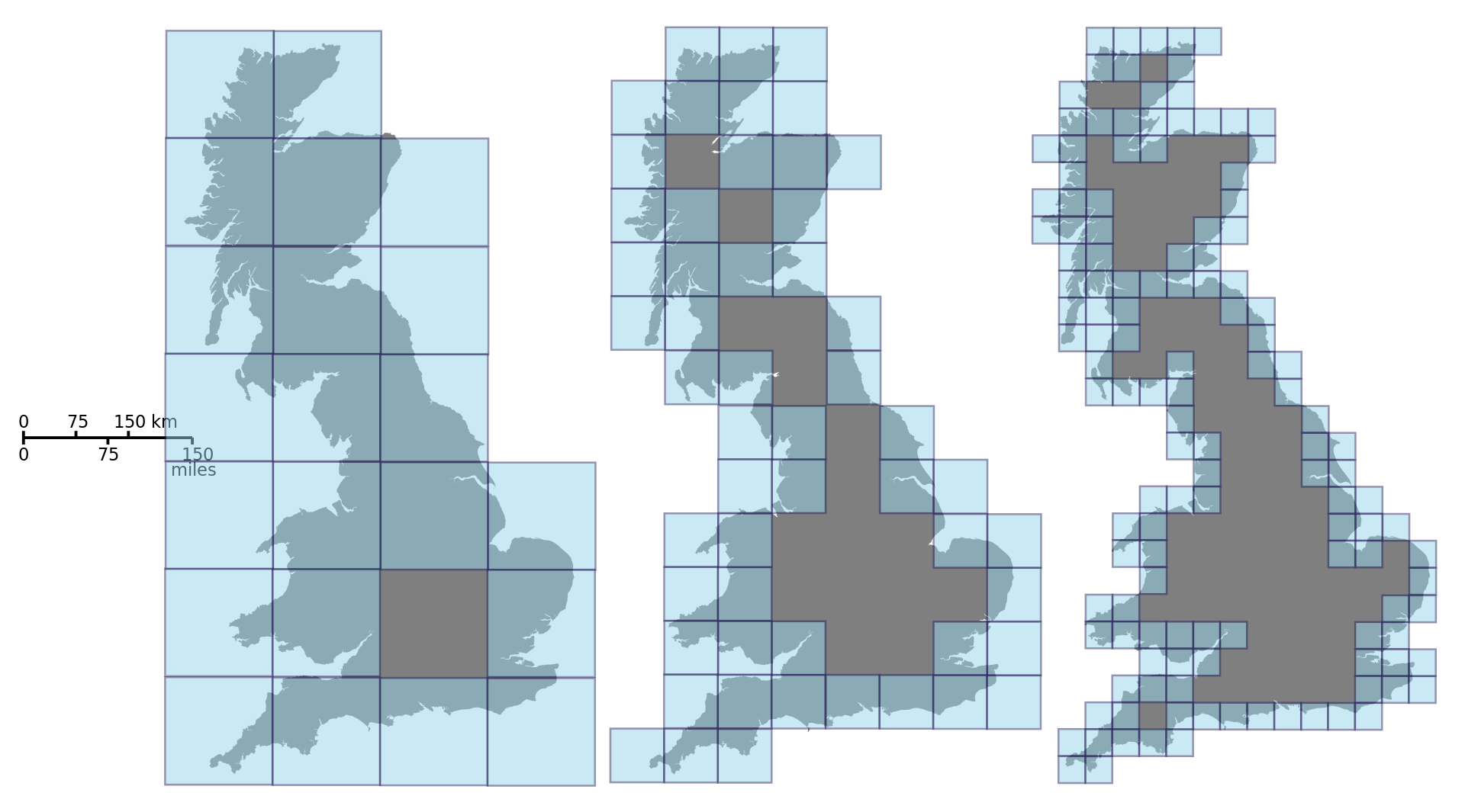
The box-counting algorithm is the most popular method of fractal analysis. It consists of defining scanning boxes (of a square shape) with exponentially increasing sizes and scanning through a binary image. If an edge is detected inside the current box, a count is added to the total.

This can be easily generalized to three dimensions substituting squares for cubes.

By Prokofiev - Own work, CC BY-SA 3.0, https://commons.wikimedia.org/w/index.php?curid=12042116

This count is performed for each box size and the box slides through the image with a predefined stride, in our case, the stride was defined as half the box side. Using pytorch AvgPool3d function, we can detect edges as follows: if the average pooling is 0, there is no edge; if it’s 1, the object completely fills the box, without edges. Thus, a pooling between 0 and 1 means that there’s an edge. This can be achieved with the following code:

stride = (int(size/2), int(size/2), int(size/2))
pool = AvgPool3d(kernel_size = (size, size, size), stride = stride, padding = int(size/2))
# Performs optimized 3D average pooling for box-counting
S = pool(image)

Where size is the dimension of the image.

Fractal Dimension

The fractal dimension is an estimate of the complexity of a fractal as a function of scale. That is, it measures how complex the pattern is by using progressively smaller scales. You should check the Wikipedia page for fractal dimension if you want to know more.

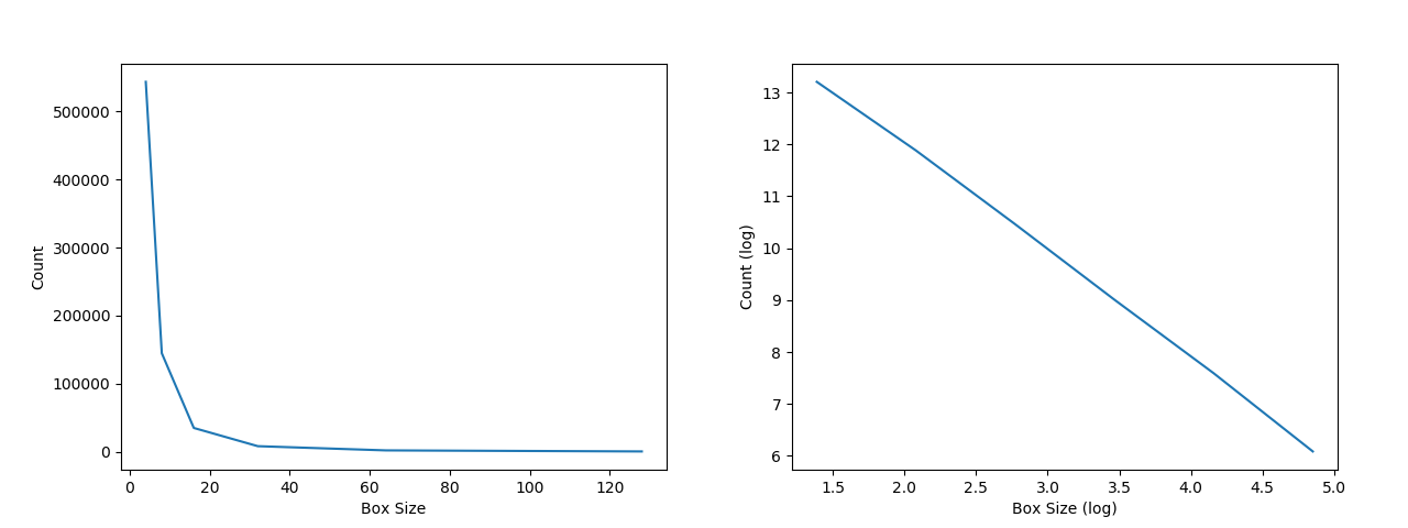
An estimator of the fractal dimension of an image can be obtained through the box-counting algorithm: the counts should follow a power law distribution in perfect fractal images, that is, the number of counts increase exponentially as the box size goes down. The fractal dimension estimator from box-counting (Db) is the opposite of the slope of a linear reggression that takes as inputs the natural log of counts and the natural log of box sizes. Applying the log transformation to both axis transforms a power law relationship into a linear one. The next two images show the effect of the log transformation:

Lacunarity

Lacunarity is another useful measure to explore fractal-like patterns. It is a measure of “gappines” and, more generally, of heterogeneity (rotational invariance). Intuitively, it can be thought as a measure of how dense a pattern is and how self-similar it is when subjected to spatial transformations. It can be estimated with the box-counting algorithm using the following formula:

where is the box size and g is the orientation. Moreover, and and are the standard-error and mean for pixels per box, recpectively.

Full code

The complete code for fractal analysis (implementing the Fractal class) is presented below:

from scipy.stats import linregress
from torch.nn import AvgPool3d
import torch

class Fractal:

    def __init__(self, Z, threshold = 1):

        # Set the default tensor as CUDA Tensor
        # If you don't have a CUDA GPU, remove all 'cuda' from the lines below
        torch.set_default_tensor_type('torch.cuda.FloatTensor')

        # Make the array binary
        self.Z = np.array((Z > threshold), dtype = int)

        # Get the list of sizes for box-counting
        self.sizes = self.get_sizes()

        # Perform box-counting
        self.count, self.lac = self.get_count()

        # Get fractal dimensionality
        slope, _, R, _, self.st_er = linregress(np.log(self.sizes), np.log(self.count))
        self.Db = -slope
        self.Rsquared = R**2

        # Lacunarity measures
        self.mean_lac = np.mean(self.lac)
        # 1 is added to avoid log of 0
        self.lac_reg_coeff, _, R_lac, _, self.st_er_lac = linregress(np.log(self.sizes), np.log(self.lac + 1))
        self.Rsquared_lac = R_lac**2

        return None

    def get_sizes(self):

        # Minimal dimension of image
        p = min(self.Z.shape)

        # Greatest power of 2 less than or equal to p/2
        n = 2**np.floor(np.log(p/2)/np.log(2))

        # Extract the exponent
        n = int(np.log(n)/np.log(2))

        # Build successive box sizes (from 2**n down to 2**1)
        sizes = 2**np.arange(n, 1, -1)

        return sizes

    def get_count(self):

        # Pre-allocation
        counts = np.empty((len(self.sizes)))
        lacs = np.empty((len(self.sizes)))
        index = 0

        # Transfer the array to a 4D CUDA Torch Tensor
        temp = torch.Tensor(self.Z).unsqueeze(0)

        # Box-counting
        for size in self.sizes:
            # i is a variable to perform box-counting at multiple orientations
            i = 0
            count_u = 0
            lac = 0

            while i in range(4) and ((i*(size/4) + size) < min(self.Z.shape)-1):
                temp = temp[:, i:, i:, i:]
                stride = (int(size/2), int(size/2), int(size/2))
                pool = AvgPool3d(kernel_size = (size, size, size), stride = stride, padding = int(size/2))
                # Performs optimized 3D average pooling for box-counting
                S = pool(temp)
                count = torch.sum(torch.where((S > 0) & (S < 1), torch.tensor([1]), torch.tensor([0]))).item()

                # Add to box counting
                count_u += count

                # Calculate Lacunarity
                u = torch.mean(S).item()
                sd = torch.std(S, unbiased = False).item()

                # 0.1 is added to avoid possible error due to division by 0
                lac += (sd/(u+0.1))**2
                #print(lac)
                i += 1

            # Avoid division by 0
            if i != 0:
                count_u *= 1/i
                lac *= 1/i

            # Results are given as an average for all orientations
            counts[index] = count_u
            lacs[index] = lac
            index += 1

        return counts, lacs

First, the array is converted to a binary one according to a provided threshold. Following, the get_sizes function calculates box sizes as powers of 2, without exceeding half the size of the array’s smaller dimension.

The get_count function performs the magic. The while loop ensures that a maximum of 4 orientations is used for each box size to decrease bias. Then, the AvgPool3d combined with the torch.where functions perform the box-counting, which is added to the count_u variable for each iteration. Also, for each iteration, a lacunarity value is calculated. The final count value is just the sum of all orientations for each size, while the final lacunarity value is the average for all orientations at a given box size.

The fractal shown in the GIF image has a 2.05795 fractal dimension and a 1.19497 mean lacunarity. If you want a more in-depth view of fractal analysis, consider reading this article.