
Over the last 100 years, p-values have become increasingly common in many scientific fields, after its development by Ronald Fisher around 1920. Now, on the aproximate 100th anniversary of the all-famous p-value, its use is being questioned due to irreproducible research, p-hacking practices and various misunderstandings about its true meaning.
Reporting only p-values is becoming less acceptable, and for good reason. Scientists should also report full data distribution, confidence intervals and details about the statistical test used and its assumptions. Those who continue to report only that P < 0.05 will face more and more questions from journals and reviewers. All this is good for science and open science. Still, p-values are very useful and will not disappear - at least not for now.
But what exactly is a p-value? Many scientists have never thought about this question explicitly. So, let’s define the p-value and then look at what it is not. Defining what something is not is a great wat to remove misconceptions that may already be lurking in our heads.
The American Statistical Association defines the p-value as:
[…] The probability under a specified statistical model that a statistical summary of the data (e.g., the sample mean difference between two compared groups) would be equal to or more extreme than its observed value.
American Statistical Association — ASA Statement on Statistical Significance and P-Values
Most often, the specified statistical model is the null hypothesis: H0 or the hypothesis that group means (or another statistical summary, such as median) are not different. Or that the correlation between two continuous variables is not different from 0. I guess 99% of the times we encounter p-values it’s under these circumstances.
So, the p-value is the probability that, given that H0 is true (this is extremely important), the results would come up with at least the difference observed.
Let’s look at what p-values are not:
1) The probability that the results are due to chance
Probably the most common misconception regarding p-values, it’s easy to see why we fall into this statistical trap. Assuming that there is no difference between the two groups, all the observed difference is due to chance. The problem here is that p-value calculations assume that every deviation from H0 is due to chance. Thus, it cannot compute a probability of something it assumes to be true.
P-values tell us the probability that the observed results would come up due to chance alone assuming H0 to be true, and not the chance that the observed results are due to chance, precisely because we don’t know if H0 is true or not. Pause and think about the difference between these two statements. If the difference is not clear, it may become clearer with the next topic.
2) The probability that H1 is true
This is a bit tricky to understand. H1 is the alternative hypothesis, in contrast to H0. Almost always, H1 states that the groups are different or that an estimator is different from zero. However, p-values tell us nothing about H1. They tell us $P(observed\ difference \vert H0)$, or the probability of the observed difference given that H0 is true. Since H0 and H1 are complementary hypotheses, $P(H0) + P(H1) = 1$. Thus, $P(H1) = 1 - P(H0)$.
However, we do not know P(H0) since we assume H0 to be true. Let’s use an example.
Let’s assume we are a patient doing blood tests for a disease called statisticosis. We know that, if you’re ill, the test returns a positive result 99% of the time. Also, if you’re not ill, it returns a negative result 98% of the time. 1% of the population is estimated to have statisticosis. Let’s assume a population of 1 million people and build a table. First, there are 990,000 people (99% of the population) without the disease and 10,000 people (1%) with the disease. Of those that are ill, 9,900 (99% of the ill) will get a positive result at the test, while 9,900 people that are not ill will also get a positive result (2% of those who are not ill).
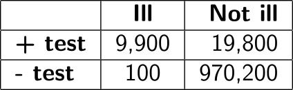
Here, H0 is that we’re not sick, while H1 is that we are sick. The probability of getting a positive result given that we are not sick is $P(+ \vert H0) = \frac{19800}{(970200 + 19800)} = 0.02$ or 2%. This is how we usually think about blood tests and its comparable to what p-values estimate: we assume H0 (not sick) to be true and calculate the probability of an observation at least as extreme as the one observed (in this case, the probability of a positive result). This number tells us that, given that we’re not sick, a positive result is unlikely (2%). However, the probability that one is not sick given a positive result is $P(H0 \vert +) = \frac{19800}{(19800 + 9900)} = \frac{2}{3}$ or 66%! In other words, if you were to receive a positive result, you would have a 66% probability of not being ill (false positive) and a 33% probability of actually being ill (true positive). It might seem like the test is useless in this case, but without the test, we can only know that our probability of being ill is 1% (population prevalence). This example, of course, ignores symptoms and other diagnostic tools for the sake of simplicity.
How can these two probabilities be so different? The thing here is the low prevalence of the disease. Even with a good test, there are many, many more people without the disease (compared to people with the disease), so a lot of false positives will occur.
The important thing here is to understand that $P(+ \vert H0) \neq P(H0 \vert +)$ and that these probabilities can be wildly different. This confusion is known as the prosecutor fallacy.
P-values are comparable to $P(+ \vert H0)$. We assume the null hypothesis, therefore we cannot calculate it’s probability nor the probability of H1. Therefore, p-values tell us nothing about the probability of H0 nor of H1. There is no better estimate because we do not know the probability that H1 is true before (a priori) our observations are collected. If this notion of a priori probabilities seems fuzzy, let’s look at the next misconception.
3) Chance of error
This mistake arises because we often report that a threshold of P < 0.05 was used (or that $\alpha = 0.05$). By assuming a 5% threshold, we assume a 5% type-I error rate. That is, we will wrongly reject the null hypothesis 5% of the times that the null hypothesis was true. This does not mean an overall error rate of 5%, because it’s impossible to know how many hypotheses are truly null in the first place. The proportion of true and false hypotheses being tested in a study or even in a scientific field would be the prior (a priori) probabilities we talked about. That would be like knowing how many people are ill, but it’s impossible in the case of hypothesis. We only use p-values because it’s impossible to know the proportion of true hypotheses being tested.
Thus, if we reject the null hypothesis when P < 0.05, we will wrongly do so in 5% of true null hypotheses. But we can’t know how many true null hypotheses there are in a study. Therefore we can’t assume that 5% of results will be wrong according to the p-value. It might be much more.
This is why a hypothesis must be very well-founded in the previous scientific evidence of reasonable quality. The more hypothesis are incrementally built upon previous research, the bigger the chance that a new hypothesis will be true. Raising the proportion of true hypothesis among all those being tested is fundamental. A low true-hypothesis proportion is similar to a low prevalence disease, and we’ve seen that while testing for rare events (be it hypotheses or diseases) we make much more mistakes, especially false positives! If the proportion of true hypothesis among all being tested is too low, the majority of statistically significant results may be false positives. There is even a study which explored this phenomenon and gained a lot of media attention.
Therefore, a smaller p-value does not mean a smaller chance of type-I error. The tolerated type-I error rate comes from the selected threshold, not from individual p-values. And the overall error rate comes from the accepted type-I error rate combined with sample size and the proportion of true hypothesis being tested in a study.
4) Effect sizes
Smaller p-values do not mean that the difference is more significant or larger. It just means that assuming H0 to be true that result is less likely to arise by chance.
Many measures of effect size exist to measure precisely what the name suggests: the size of the observed effect. This kind of statistical summary is really valuable because it tells us the magnitude of the observed difference, accounting for the observed variability.
An experiment with P = 0.00001 may have a Cohen’s d of 0.05, while another with P = 0.002 may have d = 0.2. Using the common 5% threshold, both are statistically significant. However, as we’ve seen, smaller p-values do not indicate the chance of error and, as we’re seeing now, nor the effect size. The latter has a higher p-value, which could make us think the effect was smaller, but the effect size is greater compared to the former (d = 0.2 vs d = 0.05).
Effect sizes should be reported because, when the sample size is big or variability is low, very small changes may become statistically significant, but the effect size is so small that it might as well be biologically irrelevant. Confidence intervals can also be calculated for effect sizes, which is another great way of visualizing magnitude and its associated uncertainty.
Conclusions
After a few examples of what a p-value is not, let’s remember what it is:
[…] The probability under a specified statistical model that a statistical summary of the data (e.g., the sample mean difference between two compared groups) would be equal to or more extreme than its observed value.
American Statistical Association — ASA Statement on Statistical Significance and P-Values
Maybe this definition makes more intuitive sense now. The point here is that p-values are very useful and will not go away soon. They should be used and are a valuable resource to make good statistical reasoning. However, they have a very strict definition and purpose, which is often misunderstood by those who apply them to their daily jobs.
Understanding what p-values indicate reminds us of the importance of well-founded hypothesis generation, of multiple lines of evidence to confirm a result, of adequate sample sizes and, most of all, of good reasoning and transparency when judging new hypotheses.
Leave a comment