Regression to the mean

Regression to the mean (RTM) is the statistical tendency for extreme measurements to be followed by values closer to the mean. In simpler terms, things tend to even out. Most of us have an intuitive grasp of this concept, but it’s useful to understand it in more depth.

Why do things tend to even out? Why do measurements tend towards the mean? When should we expect RTM to happen? Isn’t all of this too obvious? I’ll try to answer these questions here.

Why do measurements tend towards the mean?

Let’s consider a series of independent events. For instance, the score of a sequence of dart throws. Extremely low and high score are unlikely due to the typical design of dartboards. Therefore, The distribution of dart-throw scores will approximate a normal distribution.

Now, let’s consider the relationship between two consecutive dart throws. Since they are independent, we expect on average 0 correlation between their scores. Therefore, if the first throw had a high score, we couldn’t infer anything about the second throw. This is the most extreme form of RTM, since the first measurement has no influence over the second one.

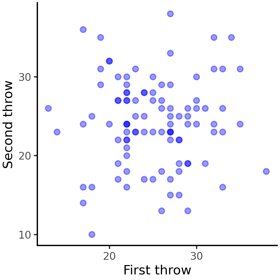
Therefore, a lucky throw doesn’t change the probability of getting extreme (high or low) scores on the next throw. The score of the second throw will be centered – of course – around the mean, regardless of the first score.

This example may seem useless, but it lies on the heart of RTM. Values tend to regress to the mean simply because the mean is the most likely value when the variable is approximately normally distributed. The normality assumption may seem restrictive, but a huge number of things are somewhat normally distributed. Even when the distribution is skewed, some form of regression still happens.

Regression between correlated measurements

Perfectly correlated variables

Consider you are a physician taking a look at patient records. You notice that for many patients there are two measurements of their height and decide to plot these two values together. Consider there is no error when measuring height. You should get something like this:

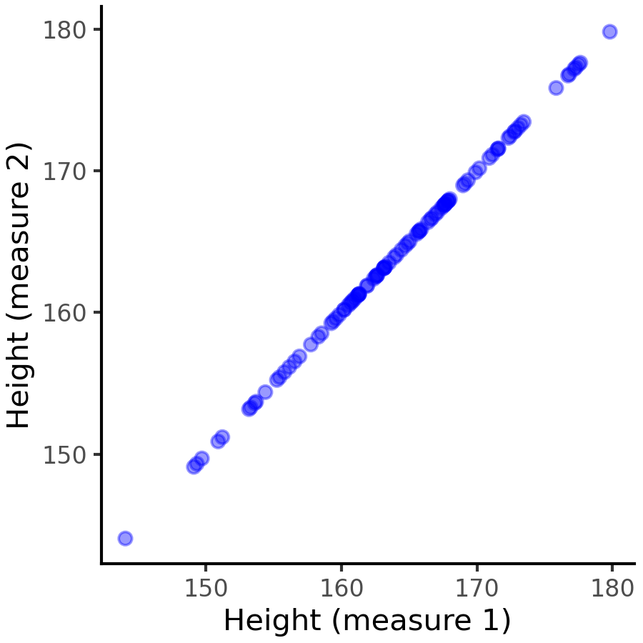
Since both measurements capture the same value (patient height), they are perfectly correlated. In this case, there is no RTM. Knowing the value of one measurement completely determines the value of the other, therefore extreme values in the first measurement remain extreme in the second one. In fact, it hardly makes sense to talk about RTM in this case, since there are no truly independent values between which the value may regress to the mean. Still, it’s important to understand that RTM doesn’t happen in this scenario and why.

The example is very specific because there are almost no (if any) two real-world measurements with perfect correlation, excluding those that express the same underlying value. Thus, almost all pairs of variables or measurements either have partial correlation or no correlation at all. When there is no correlation, we’ve seen that RTM happens at its maximum. When there is partial correlation, RTM happens with a smaller magnitude. Therefore, if you pick two random variables RTM is almost certainly at play.

Francis Galton and heights

Francis Galton first described what we now know as regression to the mean while analyzing heights of parents and children. He noticed that very tall parents usually have shorter children and vice-versa. Even though our understanding of genetics was lacking at the time, this observation laid the foundation to the concept of RTM and regression analysis more generally.

There is nothing particular about the average height that drives children towards it. Rather, due to the complex nature of heredity, the correlation between parents’ height and children’s height is not perfect and so RTM happens. Why? Well, starting with the dart throw example, the mean is the most likely value for a normal-ish distribution. Since there is a correlation, taller parents have taller kids on average. But since the correlation is not perfect, there is a significant random element, which resembles the dart throw. That is, the height of the parents only partially predict the height of the children, and the random contribution pulls values towards the mean.

There are some ways to intuitively grasp this concept. We can think that extreme values are outliers and, as such, are too unlikely to happen multiple times. Or we can think that the mean is a very reasonable most-likely value, and we drift away from the mean given a prior observation proportionately to the strength of the correlation.

Placebo effect

Even though the placebo effect is widely known, it’s often misrepresented. The placebo effect is observed in medicine and clinical trials when a placebo (an inert medical intervention, e.g. sugar pills) produces an apparent improvement of some symptoms or even objective measurements correlated with disease status. Psychological factors are relevant since a placebo may alter pain perception, for instance. But the contribution of psychological effects is not settled and, generally, there is a consensus that placebos themselves do not improve disease in any objective way.

Rather, other factors explain the observed improvement, such as RTM. There are two distinct cases: one in which the disease is expected to naturally resolve for most people, such as a common cold; another in which the disease may become or already is chronic and usually does not resolve without intervention. In the first case, the placebo effect is simply the natural course of the disease.

When dealing with chronic illness, symptoms oscillate. Let’s say we’re measuring pain. The correlation between pain in consecutive weeks is not perfect, so RTM is at play. Even with no improvement of the underlying condition, weeks of very high pain will likely be followed be weeks of more moderate (average) pain.

Patients are more likely to seek medical help or even to enroll in clinical trials when their symptoms are at their worst. This is a form of selection bias, which is another problem entirely, but it can greatly enhance the observed effect of RTM by selecting patients with unusually bad symptoms. The opposite is also true. If we actively seek patients with rheumatoid arthritis in periods of exceptionally low pain, they will likely experience more pain in subsequent weeks, regardless of the treatment.

Fooled by regression to the mean

There is nothing causal in RTM. Good test scores do not produce lower scores, terrible profits do not produce better results in the next quarter. However, it’s tempting and makes intuitive sense to interpret these phenomena as causal relationships. In fact, it’s tempting to see causality everywhere, but we should be cautious.

Whenever we make a measurement, take an action to influence it, and measure it again RTM is at play. This is commonly seen in punishment and reward strategies. Using sports results as an example, luck and other random factors are always at play, so there is imperfect correlation between two subsequent performances of the same athlete. As we’ve seen above, chances are that very bad results will be followed by better ones and vice-versa, regardless of punishment or reward.

Even though it might seem superficially simple, measuring the causal effect of any intervention is surprisingly challenging. Finding a controlled environment with as little external influence as possible is already a big challenge, but statistical phenomena such as RTM still impair our ability to reach causal conclusions. This is of extreme relevance to many fields of science. For instance, virtually all good-quality biological research uses control groups (such as placebo groups), but this is not always possible.

In order to estimate the causal effect of anything, we need to compare the world in which the intervention occurred with the world in which it didn’t. We call the latter the counterfactual world Strictly speaking, the counterfactual world doesn’t exist. When experimental designs with control groups are possible, we rely on big numbers or good sampling to assume that both groups are similar enough to be compared. But in fields such as economics and sociology it’s rarely possible to create such a control group.

Even though there are statistical workarounds for the lack of a plausible counterfactual, they are out of reach in everyday life. We should be aware that causality is hard to prove and many factors, one of which is RTM, may explain the apparent effect of our interventions.

Conclusion

Regression to the mean is everywhere. It can easily fool ourselves into seeing causality where there is none. But regression to the mean itself is not causal, that is, there is nothing causing the return to the average value – it is a byproduct of imperfect correlation.